Documentation Library
Qubic System — product manuals and technical documentation.
76 manuals
·
6 categories
Software
Software applications and simulation guides
Hardware
Motion platform hardware manuals
Tutorials
Step-by-step guides and tutorials
Product Cards
Product specification sheets and datasheets
Miscellaneous
Wallpapers and additional resources
3D Prints
3D printable models for motion platforms


QS-ACE
Backend profile setup and customization for advanced users.
1 Integration
1.1 Introduction
ForceSeatMI is a user friendly and powerful interface that allows adding a motion platforms support to any application or game (referred to as SIM in the next sections). In most applications there is no need to control the hardware directly from the SIM and the SIM can use ForceSeatMI to forward telemetry data into ForceSeatPM for further processing. This approach delegates the responsibility of transforming telemetry data to actual top table motion from the SIM to ForceSeatPM. It also simplifies the error handling that the SIM has to implement.1.2 Glossary
- SIM - an application or a game that generates telemetry data (e.g. using physics engine or reading a CSF file) and sends it to ForceSeatPM via provided set of APIs.
- top table - this is an alternative name for top frame of the motion platform.
- QubicManager - platform manager application that runs ACE and controls motion platforms.
- ForceSeatMI - API that allows the SIM to send telemetry data to the ForceSeatPM.
- ACE - an Acceleration Control Engine that implements modified classical washout algorithm.
- classical washout algorithm - it is the most widely used motion-cueing algorithm. It creates the illusion of G-forces and acceleration by generating motion over a limited range of actuators. Subsequently, the machine slowly and imperceptibly returns to its neutral position, making room for the next acceleration event.
- motion cues - name for accelerations, which exert forces on the user's body. They should convince the passengers that they are driving in a real car. The algorithms which are responsible for generating these cues are named motion cueing algorithms.
- IK - inverse kinematics.
- FK - forward kinematics.
- quick tunes - mechanism in ForceSeatPM that allows end users to quickly and safely adjust motion platform operation to their preferences without the need for understanding how the system works under the hood.
1.3 Forwarding telemetry data to the platform manager
The SIM must update FSMI_TelemetryACE periodically when vehicle physics engine generates new physics frame and then must call ForceSeatMI_SendTelemetryACE to forward telemetry data to the ForceSeatPM. Once ForceSeatPM receives telemetry data, it passes the data to ACE (Acceleration Control Engine) which calculates series of required top-table positions (motions). The ACE usually is running at higher rate than the SIM to guarantee smooth motion platform operation.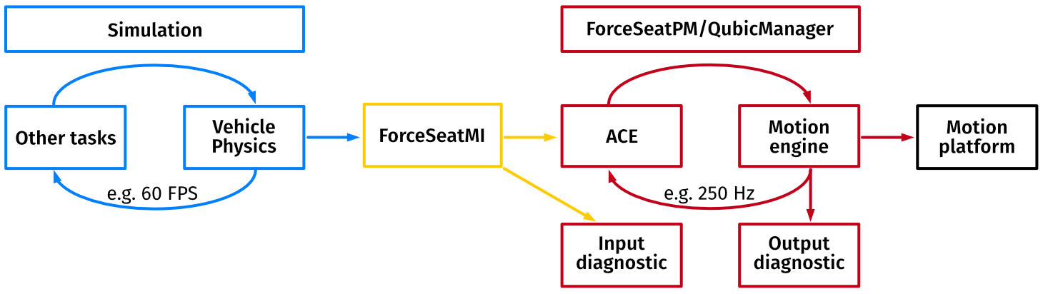
- state - indicates if the motion platform should operate or enter pause mode.
- bodyLinearAcceleration - linear accelerations in vehicle coordinate system. The accelerations might contains gravity vector.
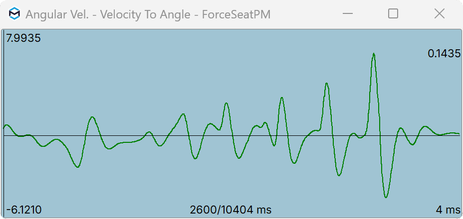
- bodyAngularVelocity - angular rotation velocity in vehicle coordinate system.
- Telemetry_CPP - it shows how to create structure in C++.
- Telemetry_CS - it shows how to create structure in C#/.NET.
- Telemetry_Matlab - it shows how to create structure in Matlab.
- Telemetry_Python - it shows how to create structure in Matlab.
- Telemetry_Fly_Unity - it shows how to get simple plane telemetry data in Unity.
- Telemetry_Fly_Unreal - it shows how to get simple plane telemetry data in Unreal Engine.
- Telemetry_Veh_Unity - it shows how to get vehicle telemetry data in Unity.
- Telemetry_Veh_Unity - it shows how to get vehicle telemetry data in Unreal Engine.
1.4 Telemetry structure
The full structure specification in C++ is presented below for reference. The same structure is available in C#, Python and Matlab formats.struct FSMI_TelemetryACE
{
// Put here sizeof(FSMI_TelemetryACE). NOTE: This field is mandatory.
FSMI_UINT8 structSize;
// Only single bit is used in current version.
// (state & 0x01) == 0 -> no pause
// (state & 0x01) == 1 -> paused, FSMI_STATE_PAUSE
FSMI_UINT8 state;
FSMI_INT8 gearNumber; // Current gear number, -1 for reverse,
// 0 for neutral, 1, 2, 3, ...
FSMI_UINT8 accelerationPedalPosition; // 0 to 100 (in percent)
FSMI_UINT8 brakePedalPosition; // 0 to 100 (in percent)
FSMI_UINT8 clutchPedalPosition; // 0 to 100 (in percent)
FSMI_UINT8 dummy1;
FSMI_UINT8 dummy2;
FSMI_UINT32 rpm; // Engine RPM
FSMI_UINT32 maxRpm; // Engine max RPM
FSMI_FLOAT vehicleForwardSpeed; // Forward speed, in [m/s]. For dashboard apps.
// Lateral, vertical and longitudinal acceleration from the simulation.
// UNITS: [m/s^2]
FSMI_TelemetryRUF bodyLinearAcceleration;
// Angular rotation velocity about vertical, lateral and longitudinal axes.
// UNITS: [radians/s]
FSMI_TelemetryPRY bodyAngularVelocity;
// Position of the user head for accelerations and angular velocity effects
// generation in relation to the top frame center. UNIT: [meters]
FSMI_TelemetryRUF headPosition;
// Additional translation for the top frame. UNIT: [meters]
FSMI_TelemetryRUF extraTranslation;
// Additional rotation for the top frame. UNIT: [rad]
FSMI_TelemetryPRY extraRotation;
// Rotation center for the 'extra' transformation in relation to
// the top frame center. UNIT: [meters]
FSMI_TelemetryRUF extraRotationCenter;
// Custom field that can be used in script in ForceSeatPM to trigger user actions.
FSMI_FLOAT userAux[FSMI_UserAuxCount];
// Custom field that can be used in script in ForceSeatPM to trigger user actions.
FSMI_UINT32 userFlags;
};
struct FSMI_TelemetryRUF
{
FSMI_FLOAT right; // + is right, - is left
FSMI_FLOAT upward; // + is upward, - is downward
FSMI_FLOAT forward; // + is forward, - is backward
};
struct FSMI_TelemetryPRY
{
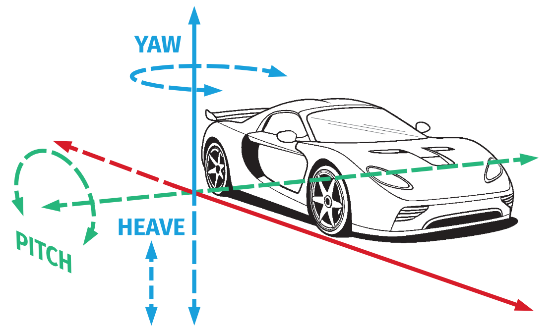
FSMI_FLOAT pitch; // + front goes up, - front goes down
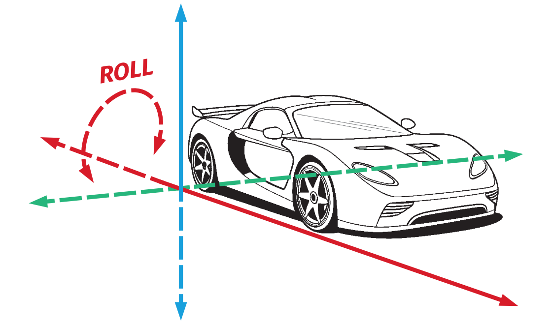
FSMI_FLOAT roll; // + right side goes down, - right side goes up
FSMI_FLOAT yaw; // + front goes left, - front goes right
};1.5 Gathering vehicle telemetry data
There are different ways of gathering telemetry data and chosen approach depends on the capabilities and interfaces of the vehicle physics engine the SIM is using. If it is possible, it is always recommended to get angular velocities and linear accelerations directly from the vehicle physics engine. Calculating angular velocities from roll/pitch/yaw changes and linear accelerations from linear velocity changes is NOT RECOMMENDED and should be used only if there is no other option.1.5.1 Suboptimal solution
Below example comes from Unreal Engine 4 example. Similar example is also available for Unity. It is also possible to get vehicle telemetry data from CSV file and then playback it or use Matlab to generate necessary data.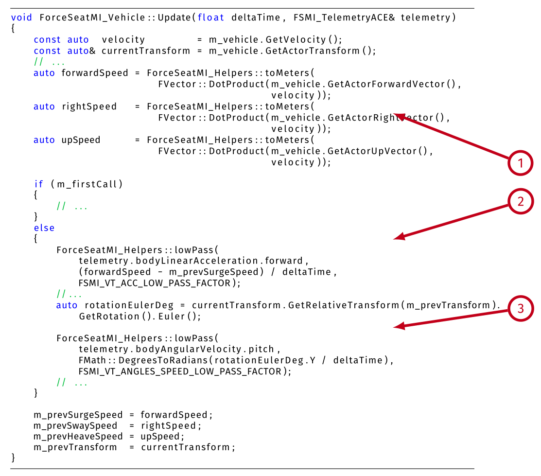
- (1) - transform object velocity from global coordinates system to vehicle coordinates system.
- (2) - calculate linear acceleration as derivate of linear velocity. This is NOT RECOMMENDED approach. If it is possible, always get linear accelerations directly from vehicle physics engine and only convert coordinates system.
- (3) - calculate angular velocity as derivate of (in this case) pitch. This is NOT RECOMMENDED approach. If it is possible, always get angular velocities directly from vehicle physics engine and only convert coordinates system.
1.5.2 Optimal solution
In this example CarSim physics engine is used and it provides an interface that allows to get linear accelerations and angular velocities directly from the engine. This is the best possible way of getting correct telemetry data. Only (optional) smoothing is performed, everything else comes directly from the vehicle physics engine.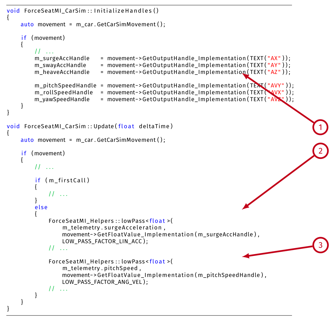
- (1) - get handles to the vehicle physics engine properties/variables.
- (2) - get linear acceleration directly from vehicle physics engine. This is a RECOMMENDED approach.
- (3) - get angular velocity directly from the vehicle physics engine. This is a RECOMMENDED approach.
1.6 Profile selection
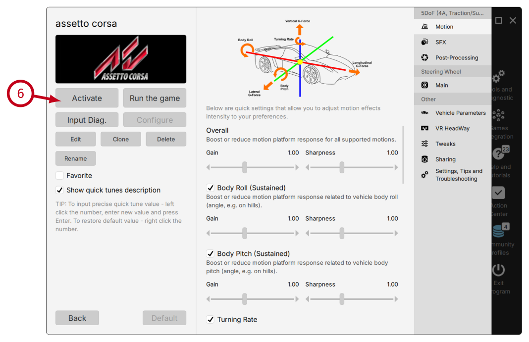
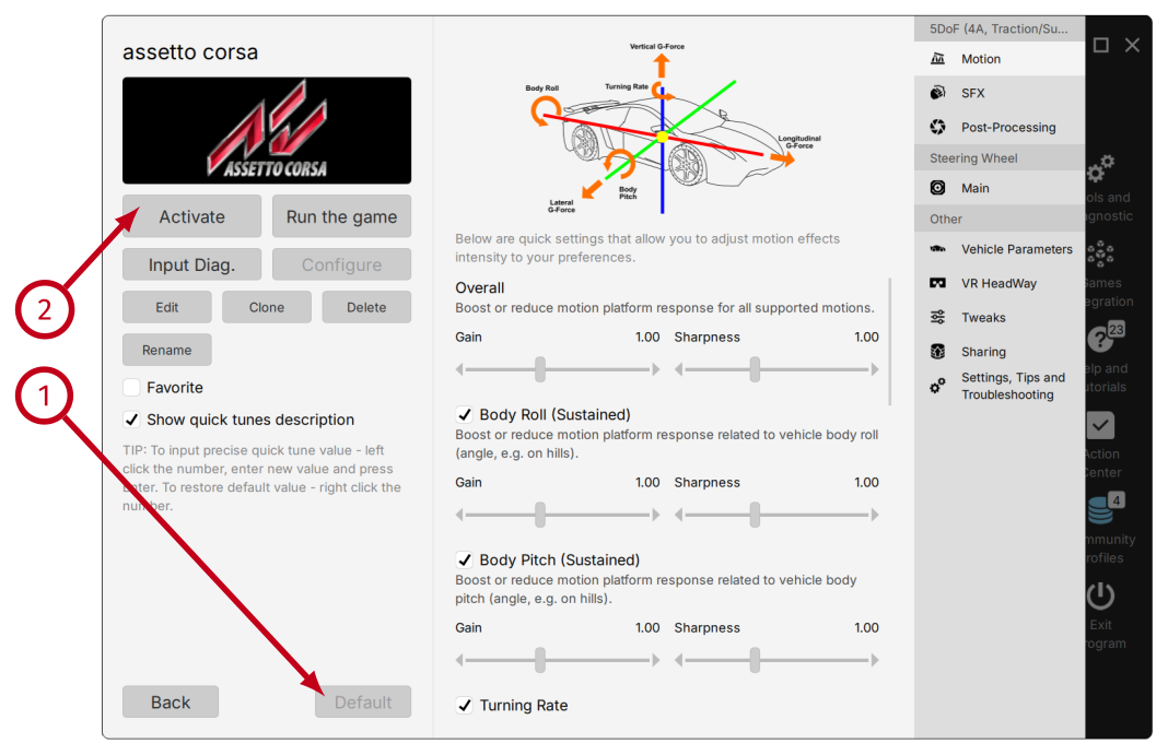
In order for the system to work, a correct profile has to be active in ForceSeatPM. For vehicle simulations it should be SDK - Vehicle Telemetry ACE (or custom profile that inherits from it). For flight simulations it should be SDK - Plane Telemetry ACE (or custom profile that inherits from it). By default all telemetry examples force ForceSeatPM to activate one of the built-in profiles. This is hardcoded in examples source code. If you want the SIM to use different profile, search source code for ActivateProfile (1) and update to use new profile name or remove completely this function call from your source code (if you want your users to change profiles themselves).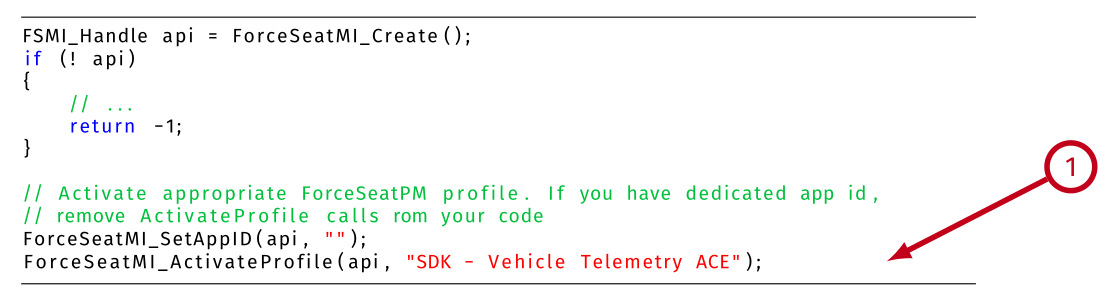
Tip
Two sets of profiles exist: SDK - Vehicle Telemetry (under Standard + user's view) and SDK - Vehicle Telemetry ACE (under ACE + user's view). The first one is deprecated and is being kept mainly for backward compatibility. For new applications it is RECOMMENDED to use SDK - Vehicle Telemetry ACE together with FSMI_TelemetryACE.
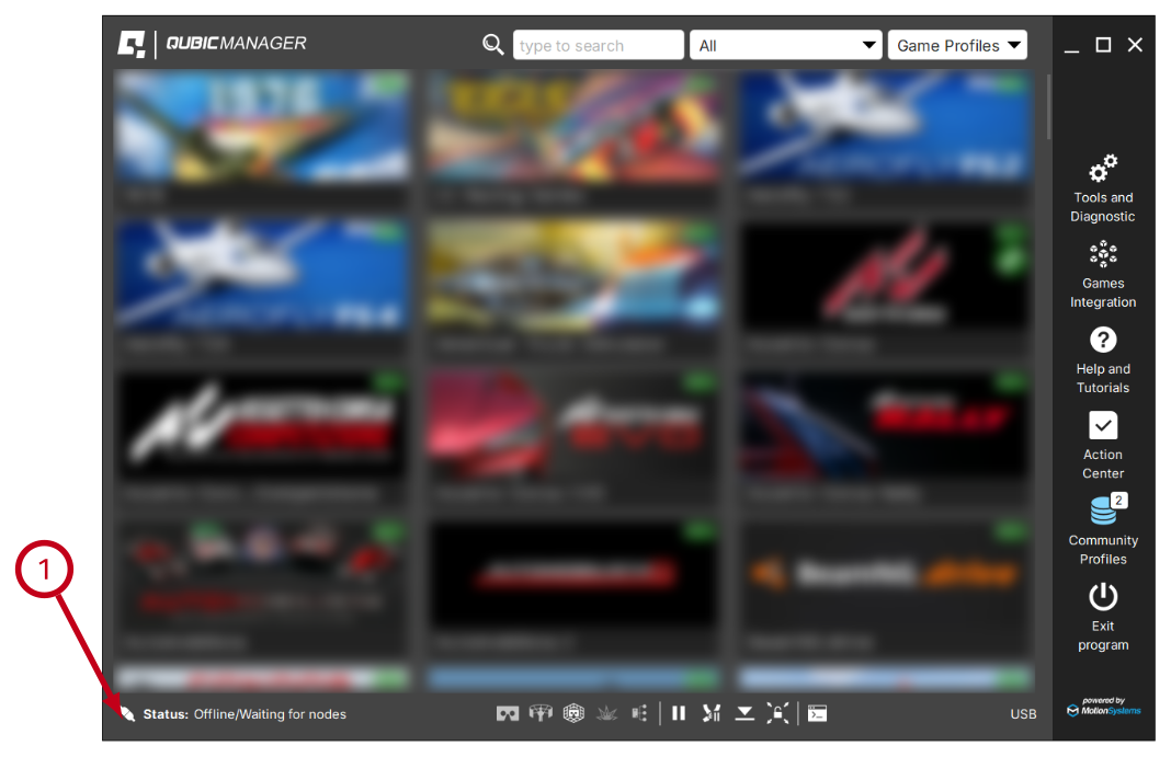
1.7 Basic diagnostic
Once the SIM has been started to send vehicle telemetry data the next step is to confirm that all necessary fields are filled correctly and that correct output to the motion platform is being generated and then sent.1.7.1 Input data diagnostic
Open profile details and click Input Diag. (1).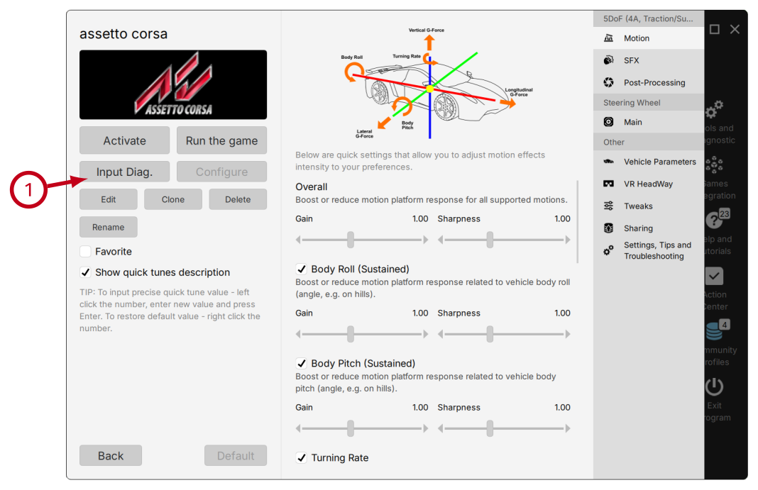
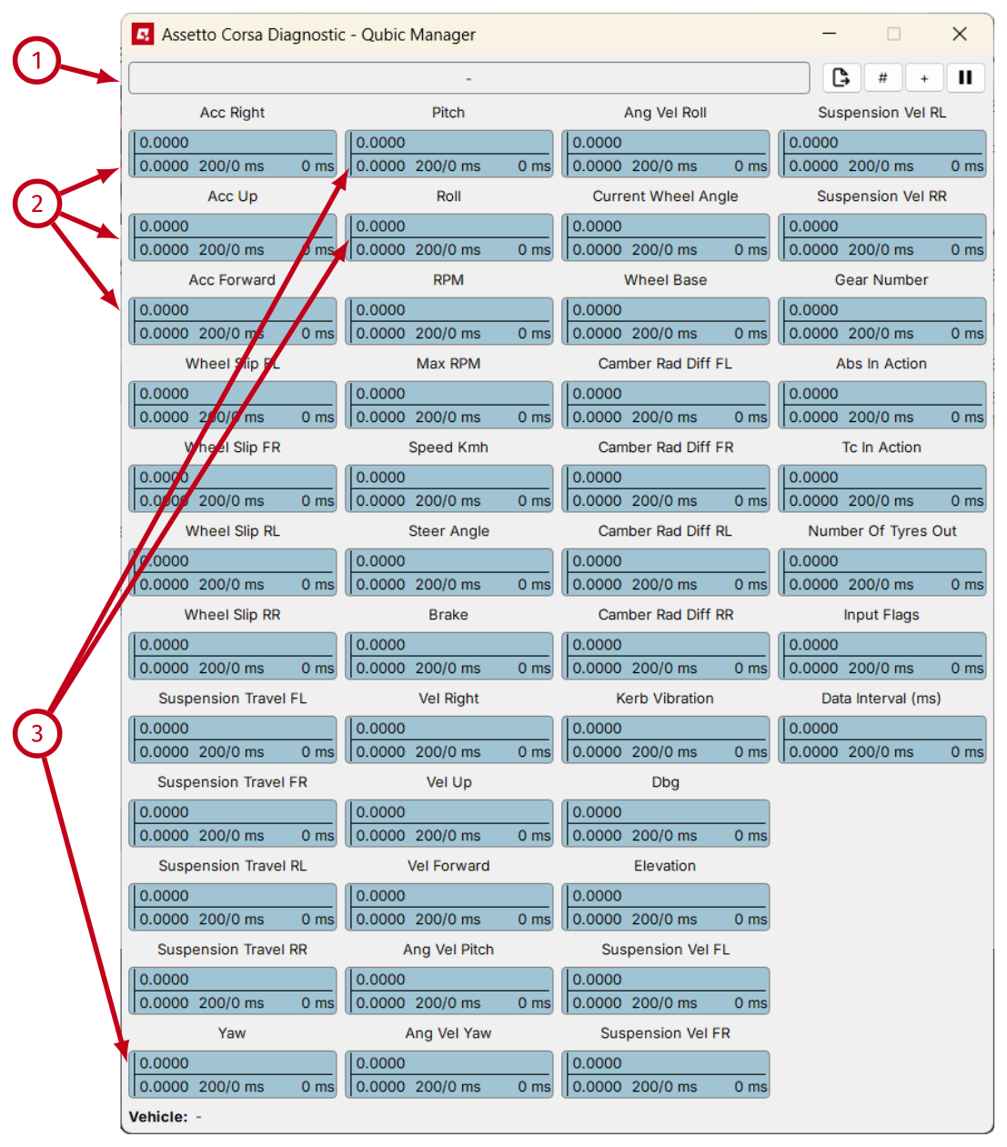
- (1) - confirm that status changes to PAUSED when the SIM is paused and returns back to RUNNING when the SIM resumes operation.
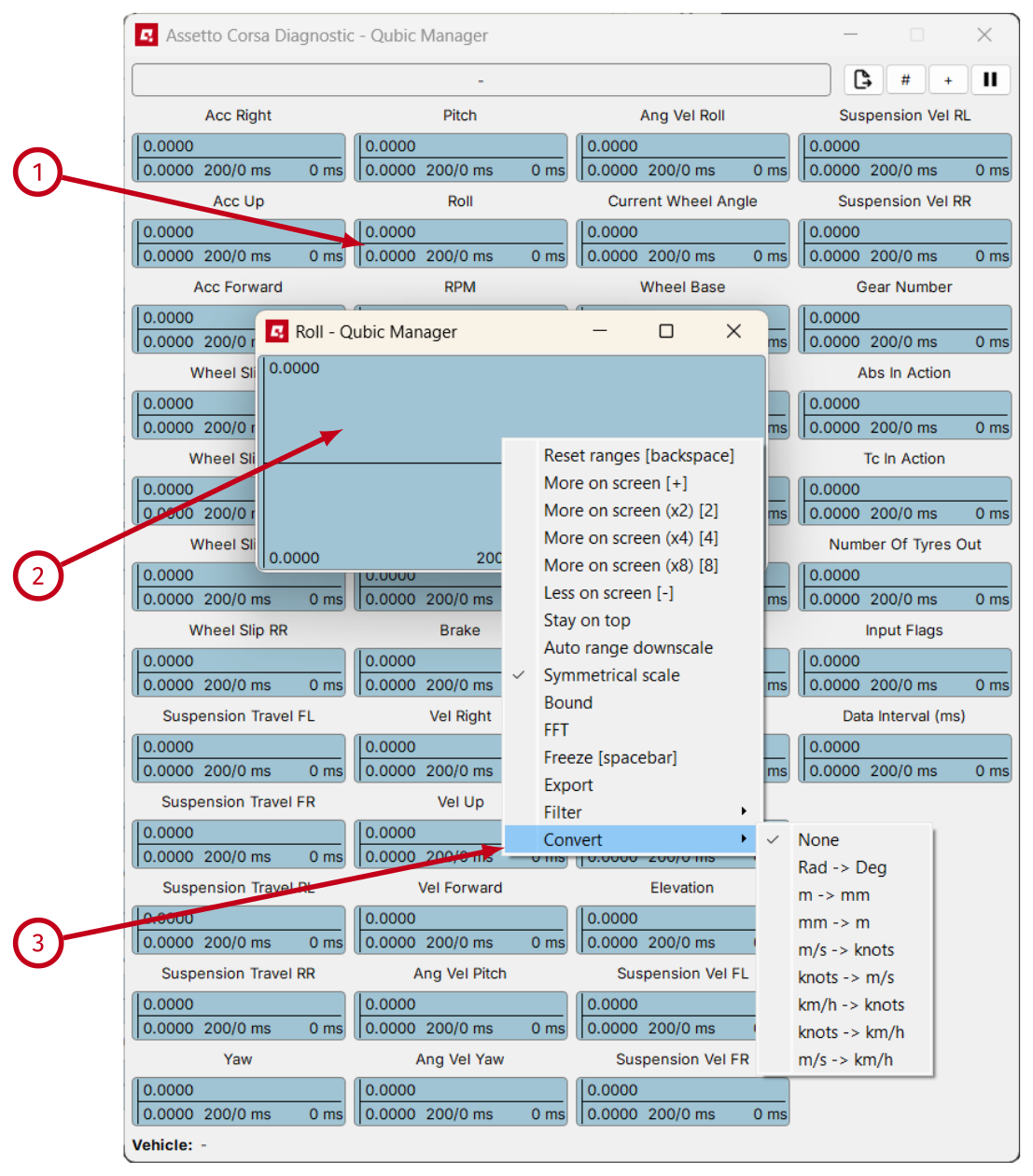
- (2) - confirm that Acc Right, Acc Up and Acc Forward are correct. You can left click on the single graph view to enlarge.
- (3) - confirm that Roll, Pitch and Yaw are correct. You can left click on the single graph view to make it bigger.
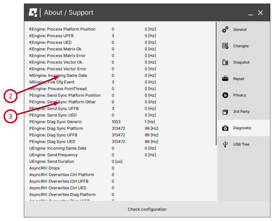
1.7.2 Input data receiving frequency
Telemetry data frequency can be checked in numerous places. First way is to check Data Interval (1) in Input Diagnostic - it will also show how the rate fluctuates.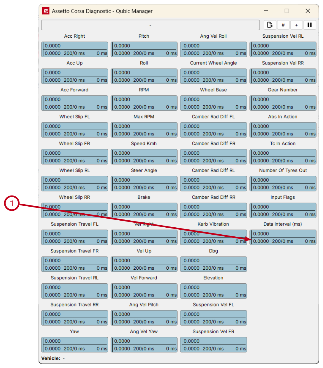
1.7.3 Required telemetry data frequency
The ACE operation frequency is independent of the SIM telemetry data rate, but there are some requirements for telemetry data rate if the SIM wants the motion platform to reproduce vibrations (embedded in linear accelerations) of specified frequency. For rectangle type vibrations (rarely used), minimal required telemetry rate is 2x the vibration frequency. For sinus type vibrations (the most common used), minimal required telemetry rate is 4x the vibration frequency.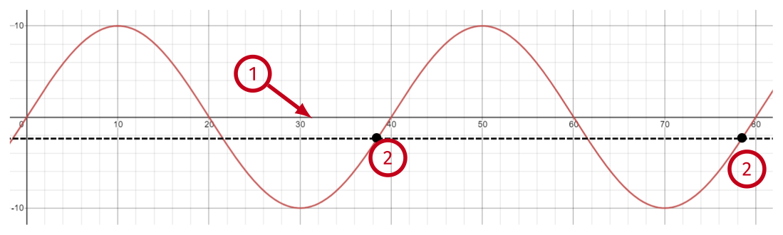
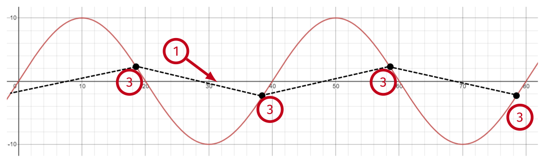
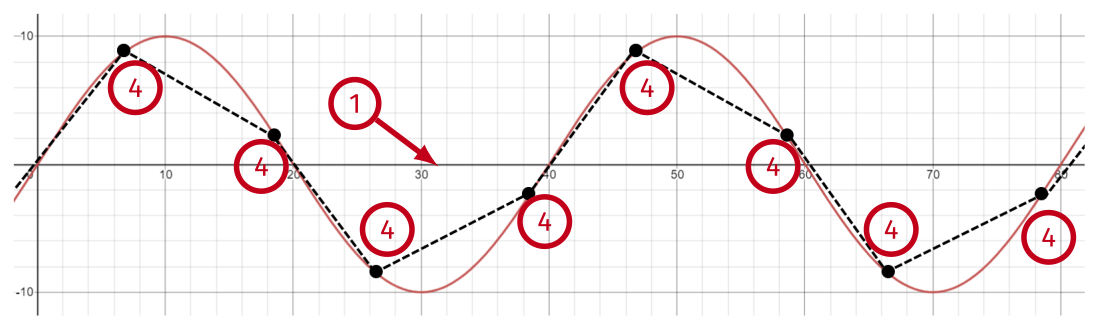
- (1) - the frequency of the vibration is 25 [Hz] which gives period of 40 [ms].
- (2) - if the telemetry rate is equal to 1x vibration rate, the ForceSeatPM receives constant signal - exact value (amplitude) depends on phase shift.
- (3) - if the telemetry rate is equal to 2x vibration rate, the ForceSeatPM might still receive value that is close to zero (or at least much less than required amplitude) - depending on phase shift.
- (4) - if the telemetry rate is equal to 4x vibration rate, the ForceSeatPM receives some approximation of the sinus which should be good enough to reproduce it on the motion platform.
ForceSeatMI_SendTelemetryACE3 is called instead of ForceSeatMI_SendTelemetryACE.
// ...
FSMI_SFX sfx;
memset(&sfx, 0, sizeof(sfx));
sfx.structSize = sizeof(sfx);

// Configure SFX
// Level 2 is supported by "PS" and "QS" motion platforms,
// Level 3 and 4 are supported by "QS" motion platforms.
sfx.effects[0].type      = FSMI_SFX_EffectType_SinusLevel2;
sfx.effects[0].area      = FSMI_SFX_AreaFlags_FrontLeft;
sfx.effects[0].amplitude = 0.05f;
sfx.effects[0].frequency = 0;
sfx.effectsCount         = 1;

// ...
ForceSeatMI_BeginMotionControl(api);
while (GetKeyState('Q') == 0)
{
	// ...
	sfx.effects[0].frequency = (byte)(sfxIterator);
	ForceSeatMI_SendTelemetryACE3(api, &telemetry, &sfx, nullptr, nullptr);
	++sfxIterator;
	if (sfxIterator > 50)
	{
		sfxIterator = 0;
	}
	// ...
}
ForceSeatMI_EndMotionControl(api);
// ...
Warning
The SIM FPS, vehicle physical engine operation frequency and in the result telemetry sending frequency might be different when the SIM is executed under Unreal Engine editor, Unity editor or other editor. It is recommended to run the SIM as standalone pre-build release binaries when motion cueing algorithm is being tuned.
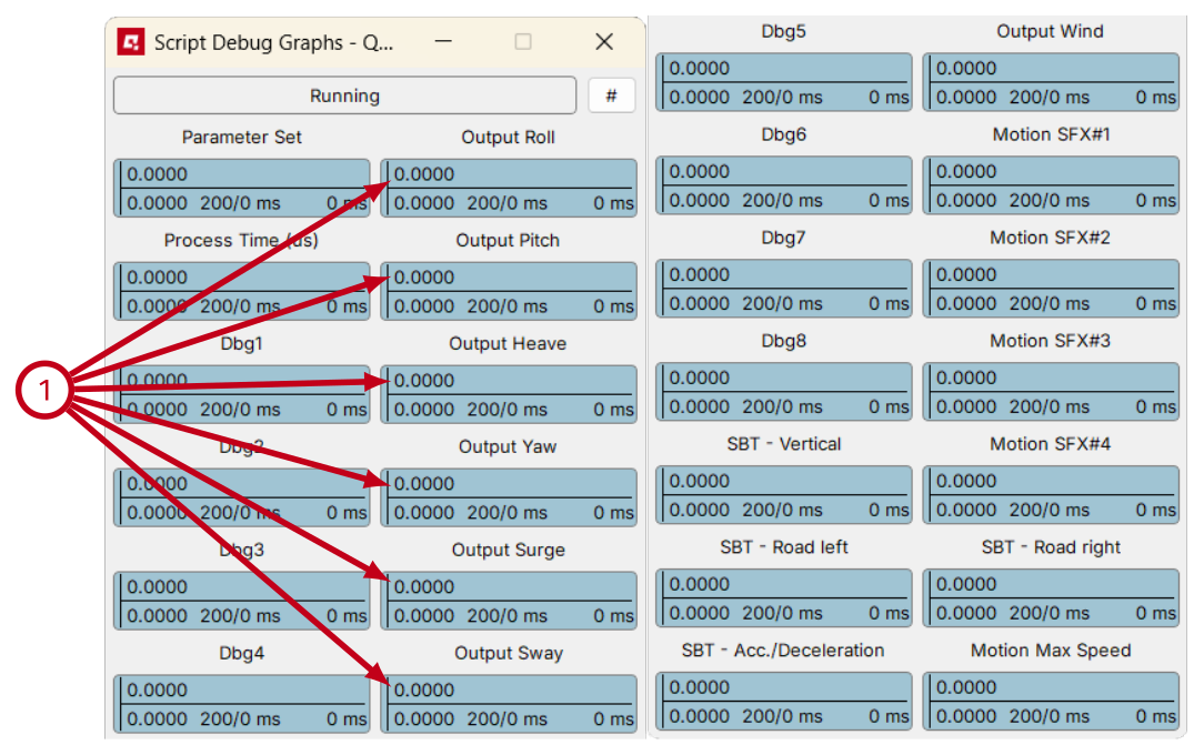
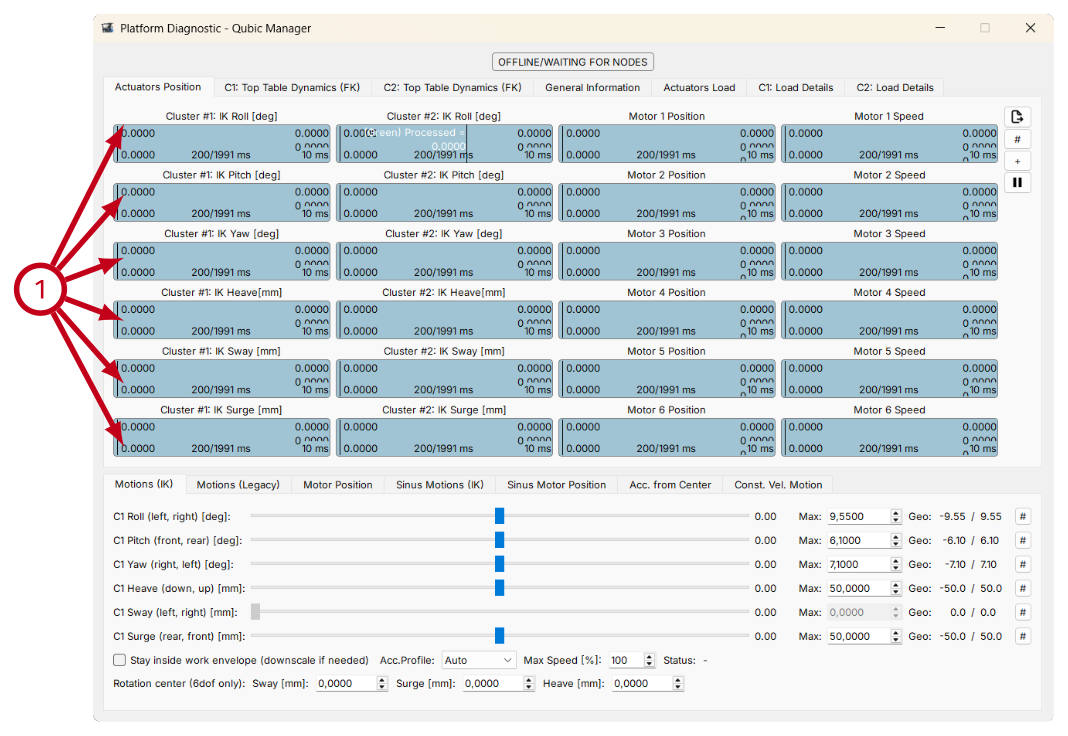
1.7.4 Output data diagnostic
Result of the motion cueing algorithm operation can be checked in following places - Script Debug Graphs (1) or in Platform Diagnostic (2).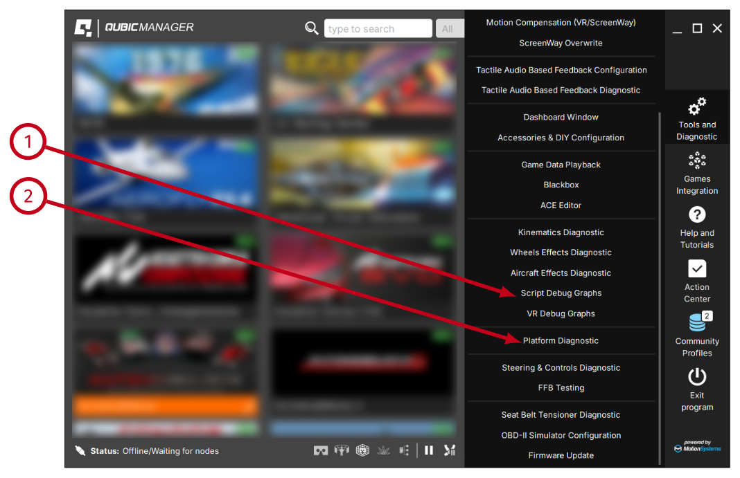
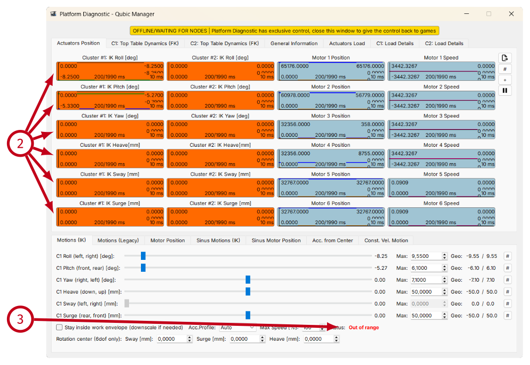
Info
It is perfectly acceptable if out-of-work-envelope issue occurs once in a while in some extreme cases (e.g. vehicle hits a wall). However if this case starts to occur too often, the motion-cueing algorithm parameters might require some adjusting.
1.7.5 Software limitations
1.7.6 Built-in profile with custom name
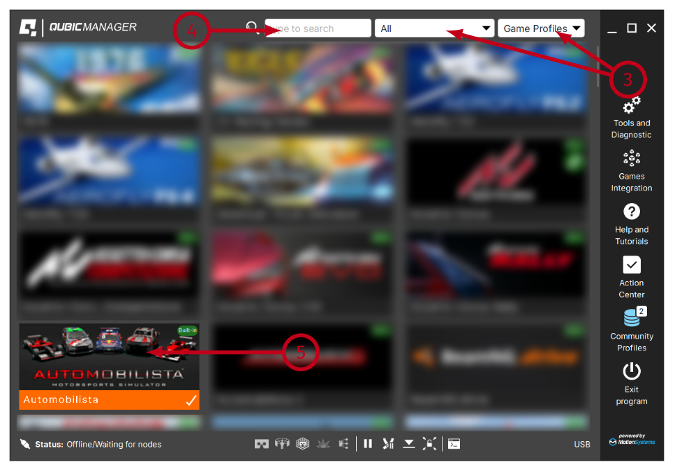
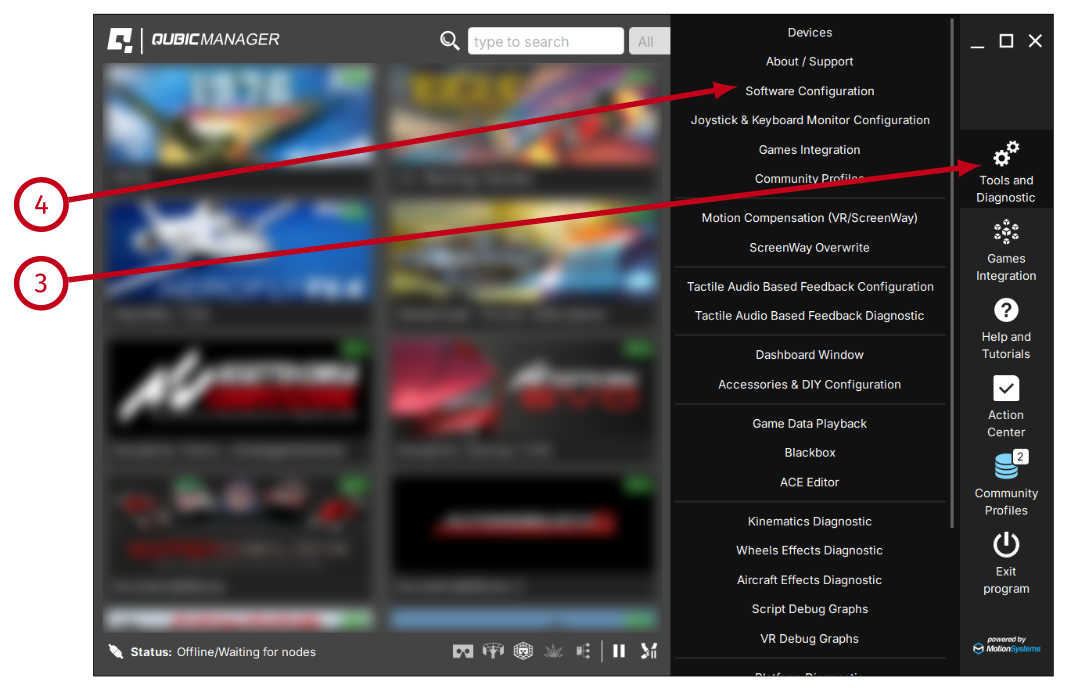
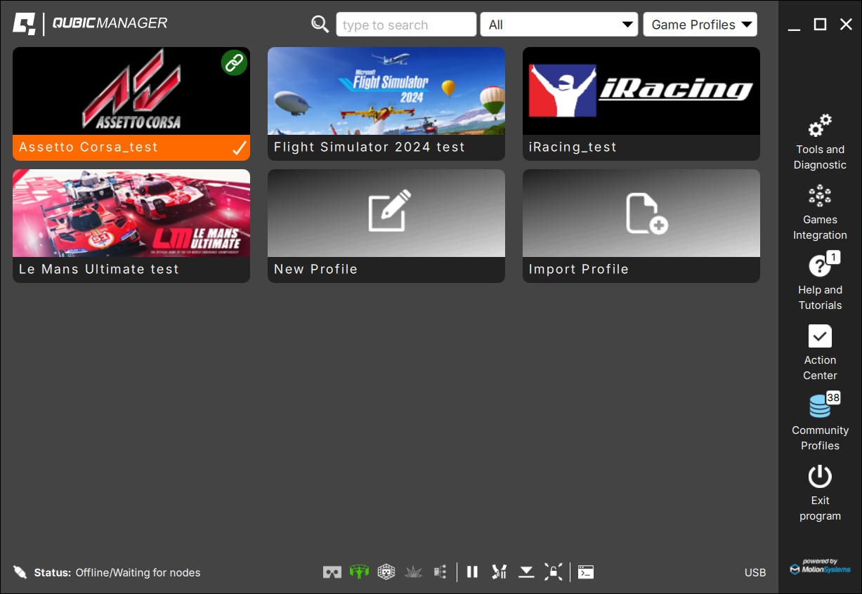
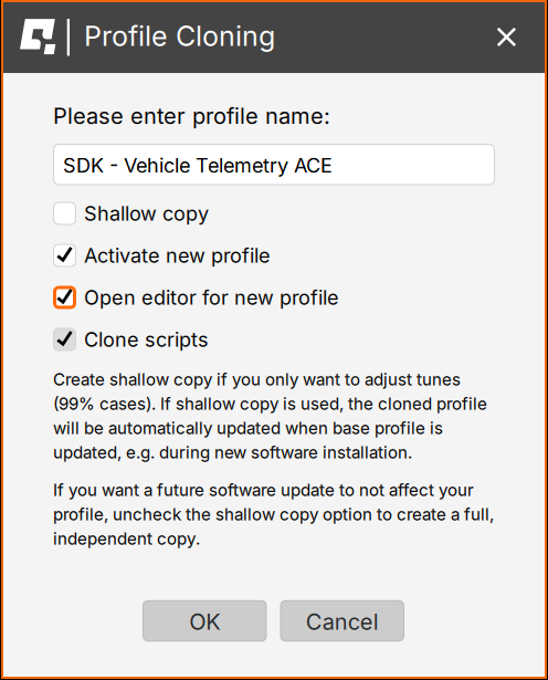
If it is required to hide all games profiles and other built-in profiles, there are a few steps that will help you to adjust the ForceSeatPM GUI to your needs. First step is to clone built-in profile (1)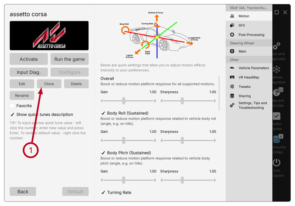
- it keeps reference to original built-in profile;
- it uses motion scripts and all other configuration from original built-in profile;
- only quick tunes values are unique for the new profile.
- changes to original profile apply also to the cloned one
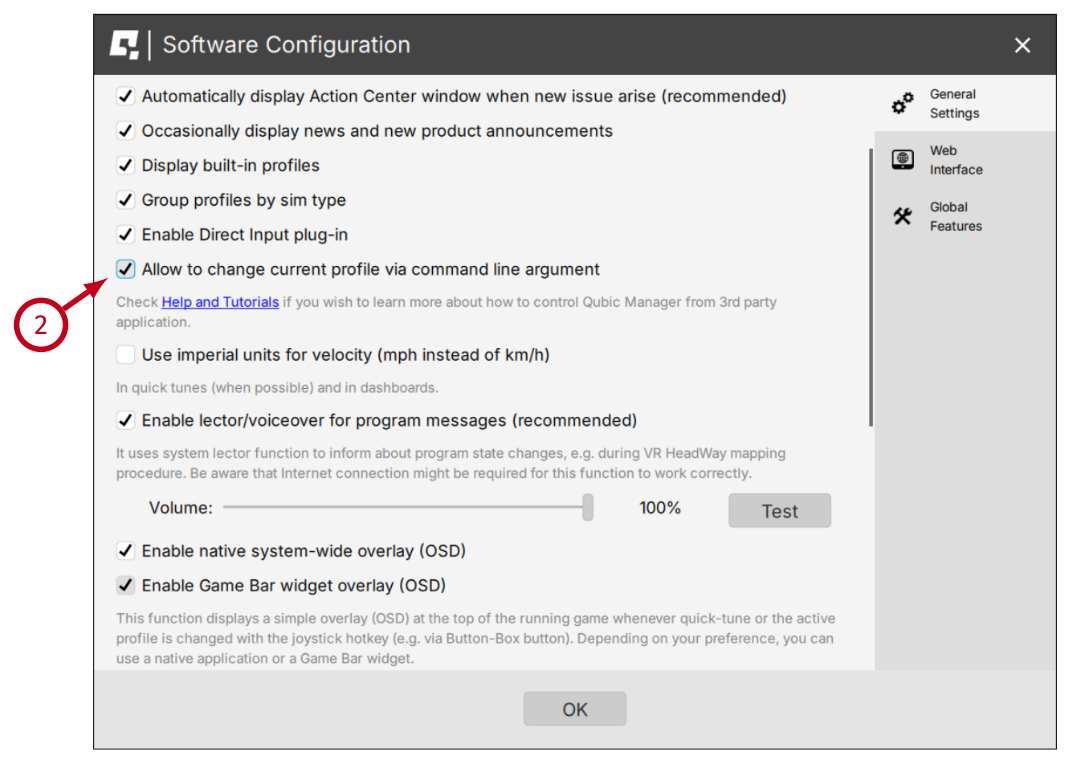
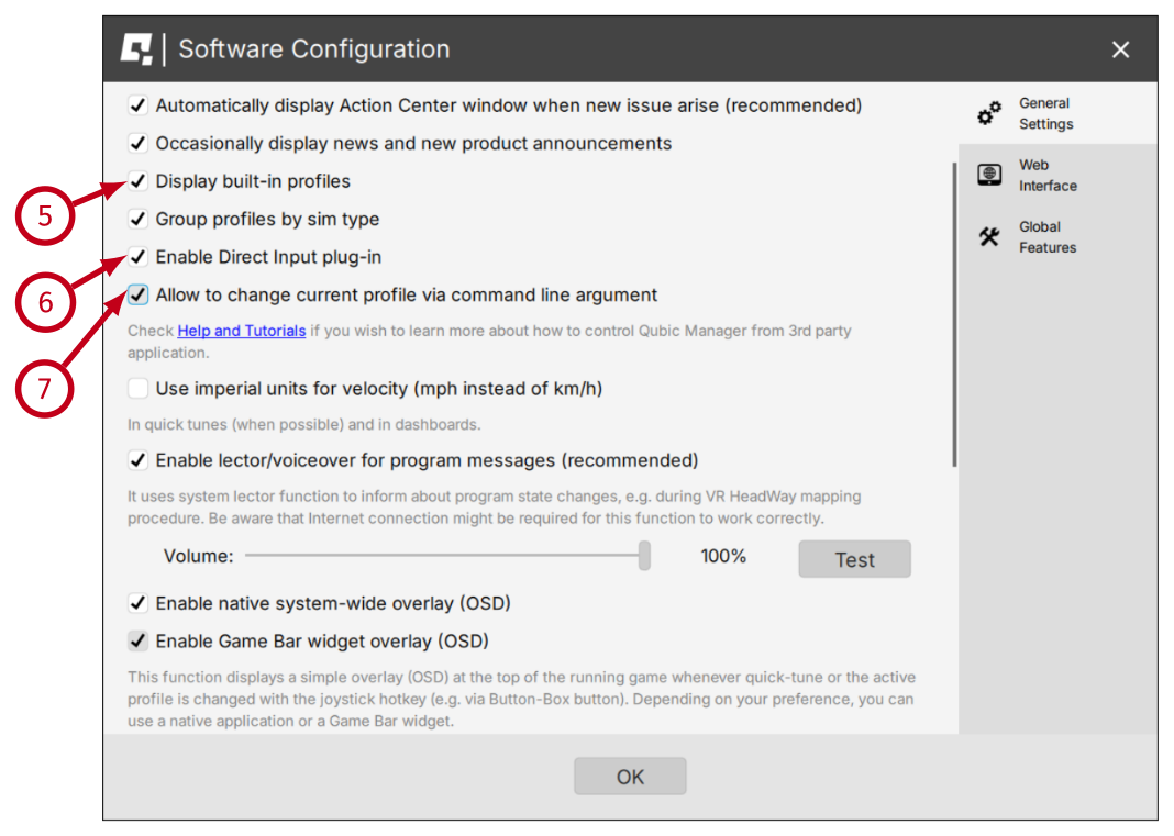
- (5) - uncheck to hide all built-in profiles and leave only your custom profiles.
- (6) - uncheck to disable option to control motion platform with joystick.
- (7) - uncheck to make sure that the SIM won't change the active profile.
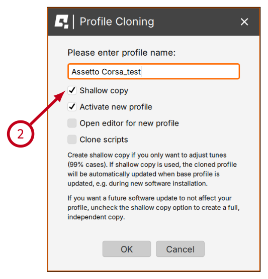
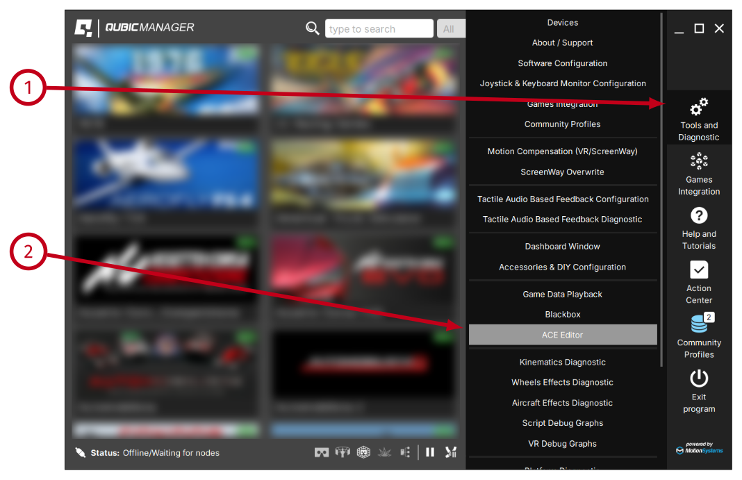
1.7.7 Editing profile with ACE Editor
The ACE configuration is stored in JSON format embedded in motion script. In order to modify it, full copy of the profile has to be made, including motion scripts cloning. The new profile will not be updated automatically when there are changes introduced to the original profile.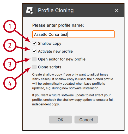
- (1) - uncheck Shallow copy
- (2) - check Activate new profile
- (3) - check Open editor for new profile
- (4) - check Clone scripts
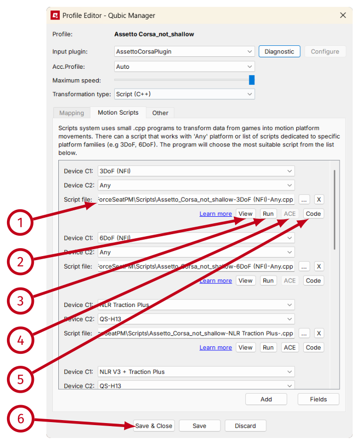
- (1) - it is the path to the motion script. There can be more than one motion script if different motion platform types (e.g. HS-xxx, QS-xxx, PS-xxx) require slightly different parameters. Having multiple motion scripts is typical scenario for games.
- (2) - it opens Windows Explorer in the directory containing the motion script.
- (3) - it runs the script to check if there are any errors.
- (4) - it loads current script to the ACE Editor.
- (5) - it opens the motion script in Visual Studio Code. This function is not used when ACE Editor is used to edit motion-cueing algorithm parameters. You can find more about Visual Studio Code in an appendix to this document.
- (6) - it saves changes (if there are any) and closes the editor.

1.7.8 Parameter sets
Warning
Keep the values of the same polarization for smooth transition between in-the-air and on-the-ground scenarios (both param sets in + or both in -).
1.7.9 Inside motion script
This document does not cover manual editing of the motion script. As a result, description of the motion script content in this section is general - its purpose is just to show what to expect in the script.Info
Motion script source code is kept in text file so it can be easily edited, even in basic notepad application. However once ForceSeatPM is ready to load the motion script, it compiles the C++ source code into native DLL and then uses only the DLL. This approach allows to combine easiness of motion script editing with high performance of C++ code compiled to native binary.
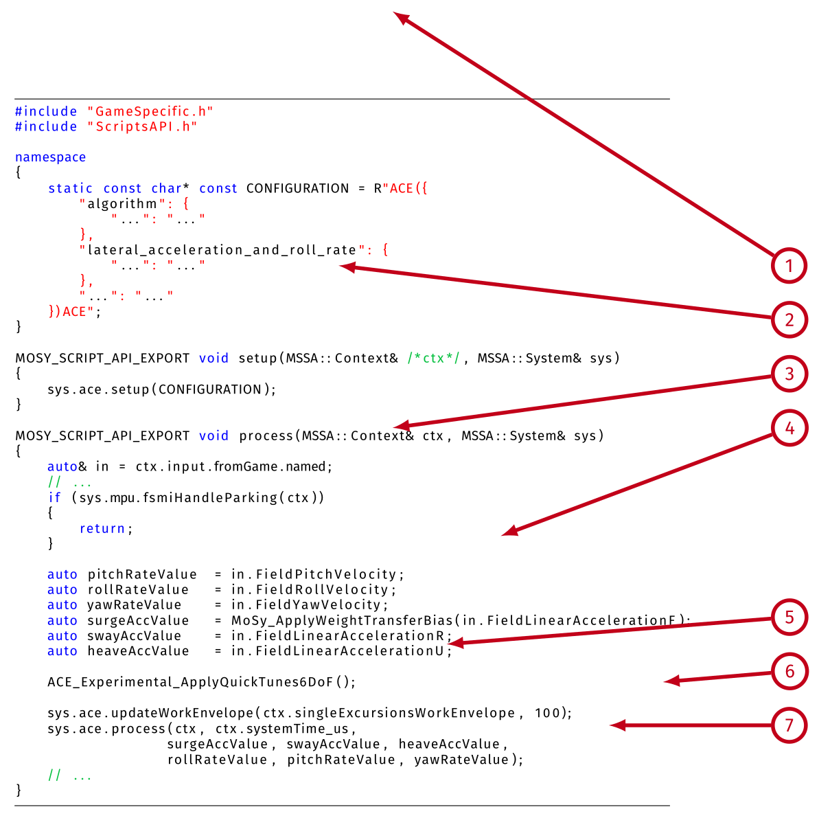
- (1) - the ACE configuration in JSON format is embedded in motion script. The ACE Editor can extract it from the motion script and then put it back.
- (2) - setup is called when the motion script is reloaded - e.g. when ACE configuration is changed - and in this case it configures ACE to use specified JSON configuration.
- (3) - process is called every ACE loop tick (not telemetry loop). This function takes telemetry data (if no new data arrived, historical are used) and then process them according the implementation. In this example, at the beginning the motion script checks if ForceSeatMI has sent parking command and if yes, there is no need to run further steps.
- (4) - assigning telemetry data to local variables is for convenience only to make optional units conversion and weight transfer bias application easier.
- (5) - it loads current values of quick tunes into ACE.
- (6) - it loads motion platform work envelope limits and scale (100%) into ACE.
- (7) - it runs the ACE.
2 Acceleration Control Engine
2.1 Introduction
ACE is an implementation of motion-cueing algorithm known as classical washout. The description of the classical washout algorithm is beyond the scope of this document. If you want to learn more, please check list of recommended articles. From https://en.wikipedia.org/wiki/Motion_simulator: "The classical washout filter is simply a combination of high-pass and low-pass filters; thus, the implementation of the filter is compatibly easy. However, the parameters of these filters have to be empirically determined. The inputs to the classical washout filter are vehicle-specific forces and angular rate. Both of the inputs are expressed in the vehicle-body-fixed frame. Since low-frequency force is dominant in driving the motion base, force is high-pass filtered, and yields the simulator translations. Much the same operation is done for angular rate. [...] Since the human vestibular system automatically re-centers itself during steady motions, washout filters are used to suppress unnecessary low-frequency signals while returning the simulator back to a neutral position at accelerations below the threshold of human perception."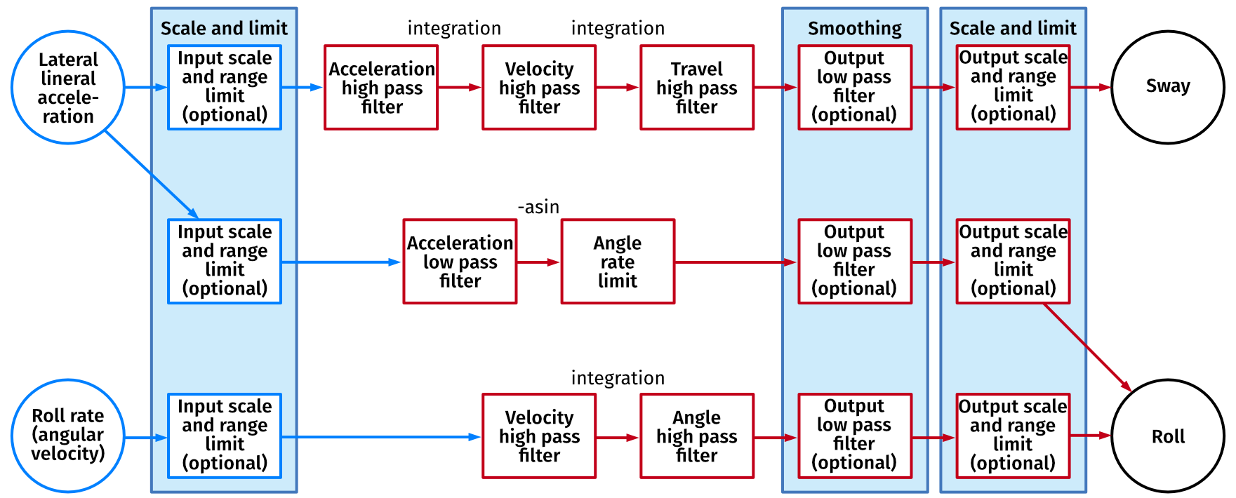
2.2 Recommended reading
In alphabetical order:- Control of a Dynamic Driving Simulator: Time-Variant Motion Cueing Algorithms and Prepositioning; Cornelius Weiß
- Development of a Full-flight Simulator for Ab-initio Flight Training with Emphasis on Hardware and Motion Integration; Jonathan Plumpton
- Implementation of a washout filter used in stewart platform; Rodrigo Lemes, Moreira De Souza, Ricardo Afonso Angélico, Ricardo Breganon, Caio Barbosa
- Motion cueing algorithms for a real-time automobile driving simulator, Zhou FANG, Andras KEMENY
- Motion Cueing Algorithms for Small Driving Simulator; Lamri Nehaoua, Hichem Arioui, Hakim Mohellebi, Stéphane Espié
2.3 Differences
The main difference between classical washout and ACE from the functionality point of view, is a presence of additional path that is not available in the classical washout algorithm. This vertical linear acceleration to pitch transformation has been introduced by MotionSystems to enable simulation of sustained vertical G during maneuvers in flight simulations (e.g. turning). It supports both positive and negative G.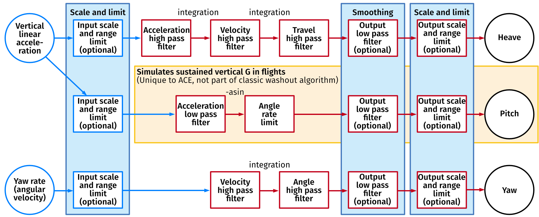
2.4 ACE and ForceSeat relation
In order to create a new profile, the user must create a clone of a Input signal generated by the game or simulation is received by the ACE software. In order for this extra path to operate correctly, the natural vertical 1g has to be removed from the vertical acceleration to avoid constant top table pitch on ground and during stable flight. This can be done inside the motion script or with usage of G1 and G2 options.MOSY_SCRIPT_API_EXPORT void process(MSSA::Context& ctx, MSSA::System& sys)
{
// Remove gravity downward force from heave to get rid of
// constant motion platform pitch on ground
auto tmpAccY = in.FieldAccY - 1.f;
// ...
auto heaveAccValue = tmpAccY * 9.81f;
// ...
sys.ace.process(ctx, ctx.systemTime_us,
surgeAccValue, swayAccValue, heaveAccValue,
rollRateValue, pitchRateValue, yawRateValue);
// ...
Tip
This feature is not used (or even needed) in vehicle (car) simulation applications.

3 ACE Editor
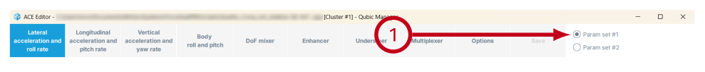
3.1 Main window
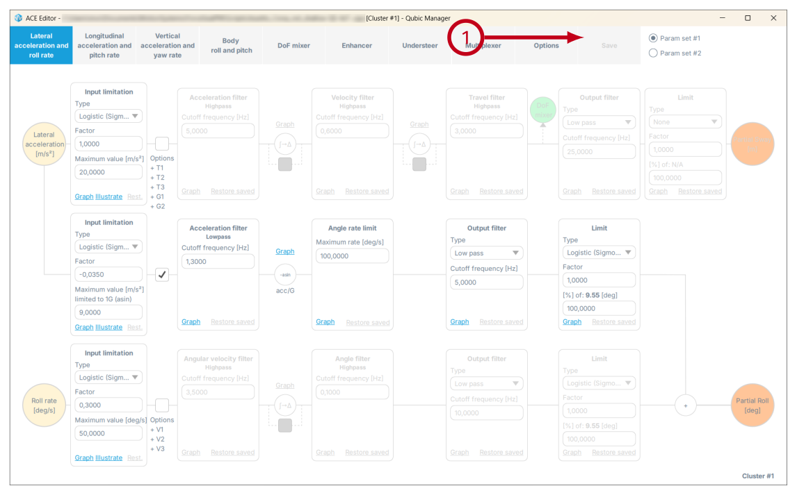
The main editor's window consists of 4 tabs, Save button and parameters set switch.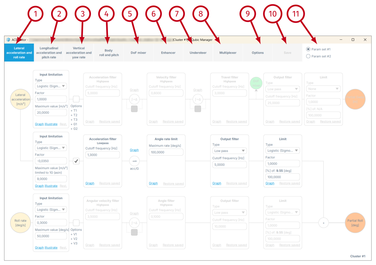
- (1) - switches to lateral acceleration and roll rate parameters.
- (2) - switches to longitudinal acceleration and pitch rate parameters.
- (3) - switches to vertical acceleration and yaw rate parameters.
- (4) - switches to body roll and pitch parameters
- (5) - switches to degrees of freedom mixer parameters
- (6) - switches to enhancer parameters
- (7) - switches to understeer parameters
- (8) - switches to multiplexer parameters
- (9) - shows global options.
- (10) - saves changes to file, which the ForceSeatPM detects and automatically reloads the motion script. You can also use Ctrl + S to save the parameters.
- (11) - switches between parameter sets. For vehicle simulations only first parameters set (#1) is used. For flights, the first parameter set (#1) is used for in-the-air scenario and the second parameters set used for on-the-ground scenario (#2). ACE interpolates values between parameters set during transition from ground to air and back. All check boxes, filter types and limits type are shared between parameters set, only numerical values can be different.
Info
In flight simulations "Param set #1" and "Param set #2" should not be polarized into negative and positive value - the transition between runway and after take-off (in-the-air scenario) will be incorrect (for example: negative values in Factor will inverse platform's movement).
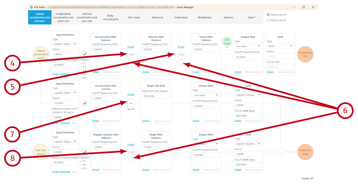
3.2 General guidelines
This section provides general guidelines and best practices to help users create a complete, accurate, and effective profile. ACE window - single tab overview: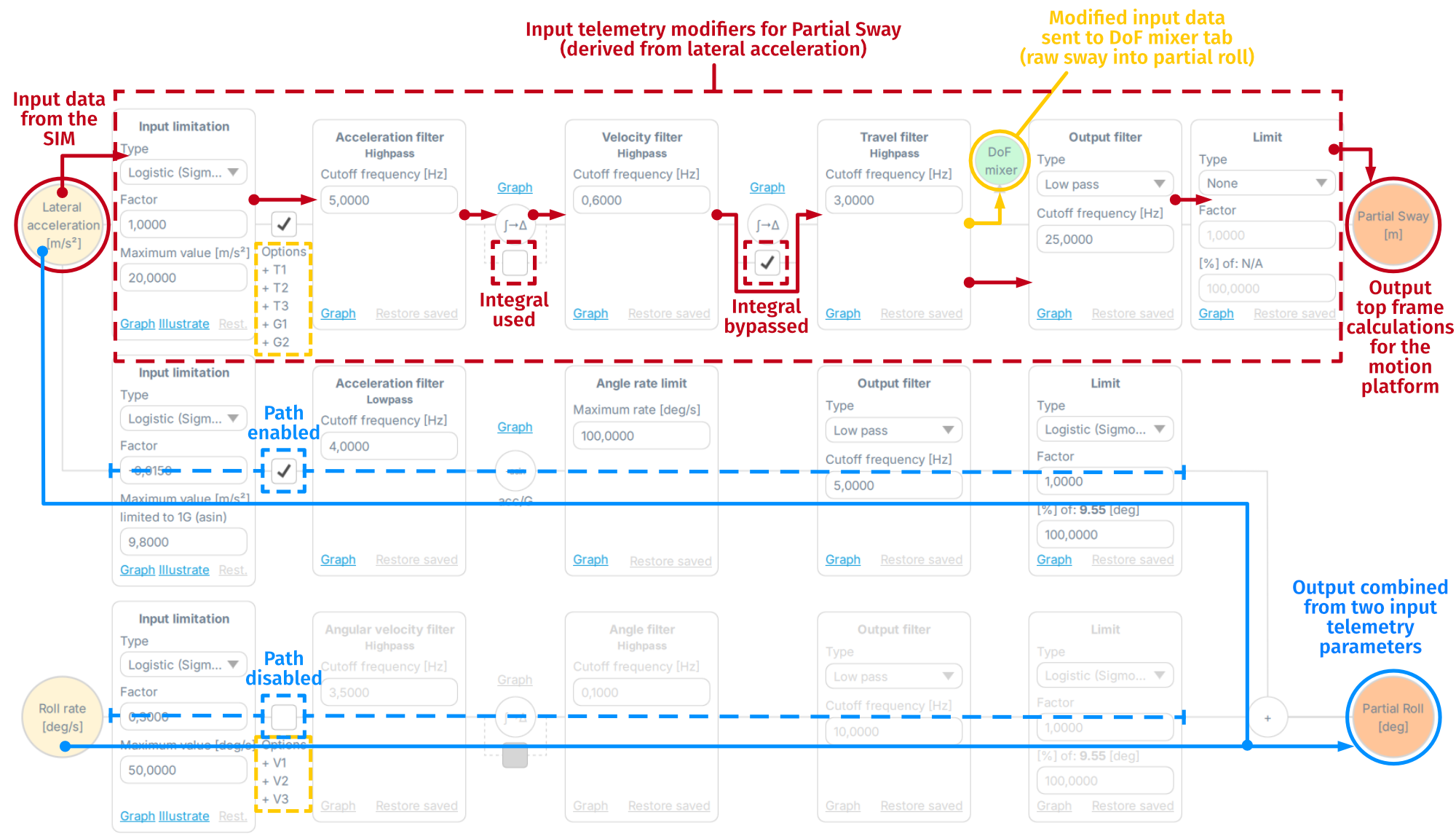
- The path from Input data to Output signal: adjusting a specific type of motion cue starts with the input parameter on the left (in this case Lateral Acceleration). It comes directly from the SIM and passes through all the blocks from left to right. Every block modifies the signal and proceeds it to the next one. Final output signal (sent to the motion platform) is symbolized by an orange circle on the right (output data). Keep in mind that the integrals are computed by default and can be bypassed - more details in section Integrals.
- The input parameter modifier path is marked by line-connected blocks: in this case a Partial Roll motion cue - the effect is combined from two input parameters - Lateral acceleration and Roll rate data. The modifying blocks affect the Partial Roll only if the path is enabled. A gray title inside an orange circle indicates that the effect is disabled (input data blocked). In this case, with Roll rate path disabled - the Partial roll motion cue draws only from Lateral acceleration input data.
- DoF mixer circle and optional transformations: the DoF mixer circle marks the signal export location from which modified data (in this case Raw sway) is sent to a separate tab to be further processed. Keep in mind that all modifying blocks are also influenced by optional transformations (+ T1, + T2, etc.). Go to Options tab to enable or disable them.
- Work in small steps - change one parameter at a time and test the result (they apply instantly after clicking "Save" button).
- Disable all output filters and limitations if you are tuning low-pass filters.
- Make sure to scale input correctly, especially for tilt coordination (e.g. lateral acceleration to roll transformation).
- Tune each path individually and then start combining them. Very often each path separately works correctly but once combined - the output motion is outside of the available work envelope or too strong.
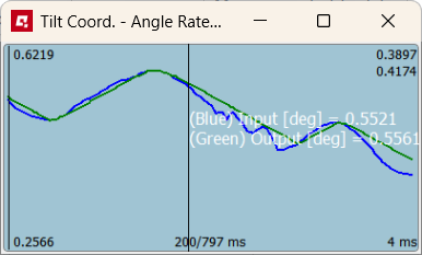
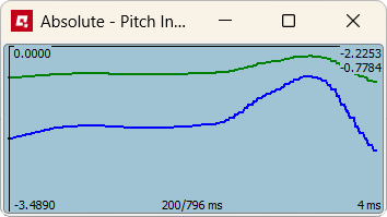
- Use graphs to visually compare input (blue line) and output (green line) signal. Right-click on the graph and select "Stay on top" to see it during gameplay/simulation.
- Start working from Input limitation block just to appropriately scale the input signal for the platform. Fine tune it using specific filter blocks later.
- Keep in mind that QubicManager and ACE interact - make sure the profile you work on is cloned and with tuning sliders in default setting (only exception is Violent Movement Suppressor - disable it to know how the platform reacts to your changes with no blockage).
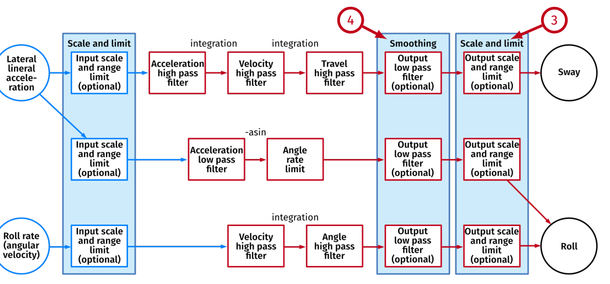
3.3 Lateral acceleration and roll rate
This view allows to configure parameters for each block of the classical washout algorithm.- lateral acceleration to sway;
- lateral acceleration to roll - known also as tilt coordination;
- roll rate to roll.
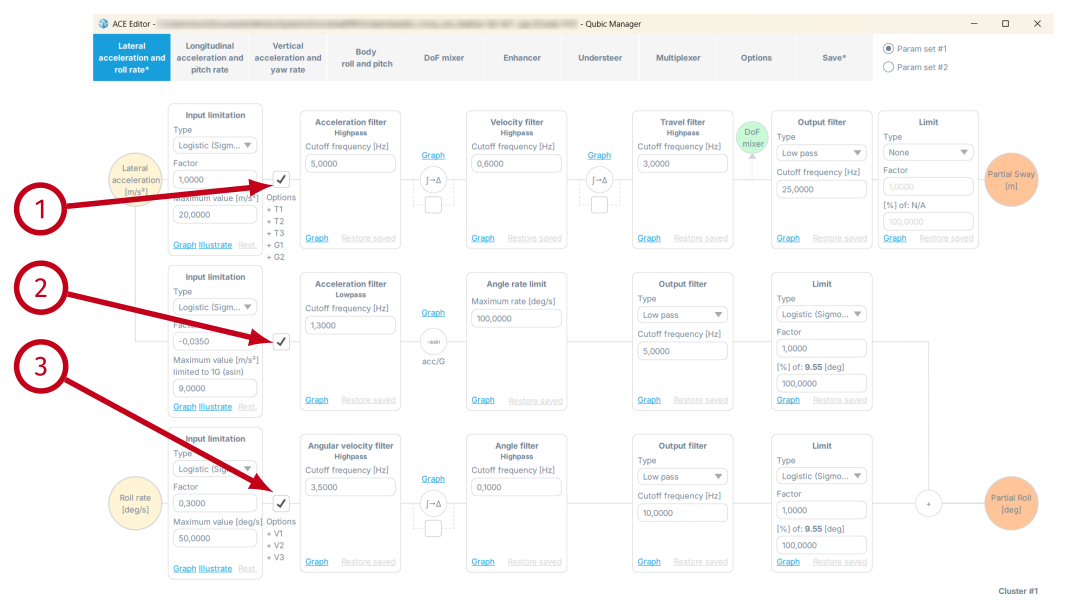
- (1) - enables lateral acceleration to sway transformation. There are optional transformations that can be applied (T1, T2, T3, G1 and G2) - go to Options tab description to learn more.
- (2) - enables lateral acceleration to roll transformation. This path is also called tilt coordination.
- (3) - enables roll rate (angular velocity) to roll transformation. There are optional transformations that can be applied (V1, V2 and V3) - check Options tab description to learn more.
- (4) - it computes integral of acceleration to get instantaneous velocity. In other words, it uses acceleration and time interval (4ms for 250Hz rate) between ACE loop calls to calculate velocity.
v = ∫00.004[s] a(t) dt
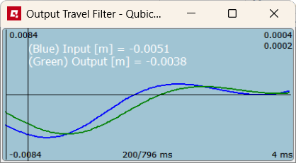
- (5) - it computes integral of velocity to get instantaneous travel. In other words, it uses velocity and time interval (4ms for 250Hz rate) between ACE loop calls to calculate travel.
s = ∫00.004[s] v(t) dt
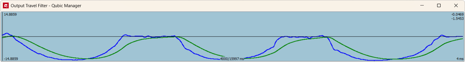
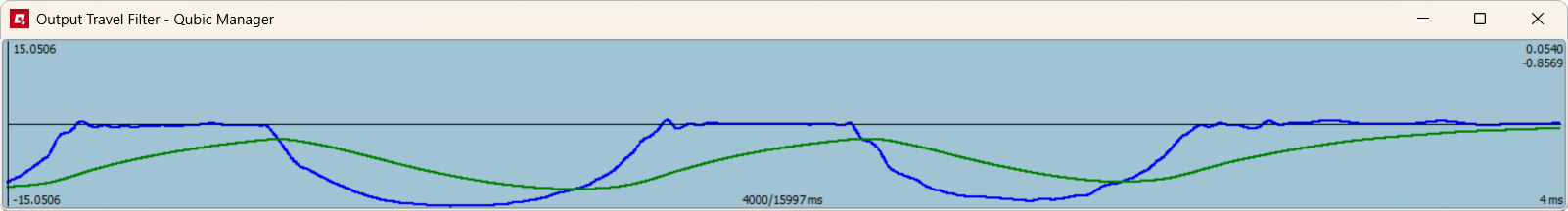
- (6) - check these boxes to bypass the integrals.
WarningIf you decide to bypass the integral, keep in mind the movement of the platform may become abrupt and intense. Examples before and after:

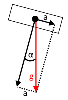
- (7) - it calculates angle of gravity vector to figure out what top table roll is required to simulate lateral force with usage of gravity force. This bases on assumption that human senses are not perfect and people are used to feel and ignore gravity when it points down. Once the gravity is felt at angle, it can be easily mistaken with lateral acceleration. This is the trick that tilt coordinate block uses.
α = -asin(ag)
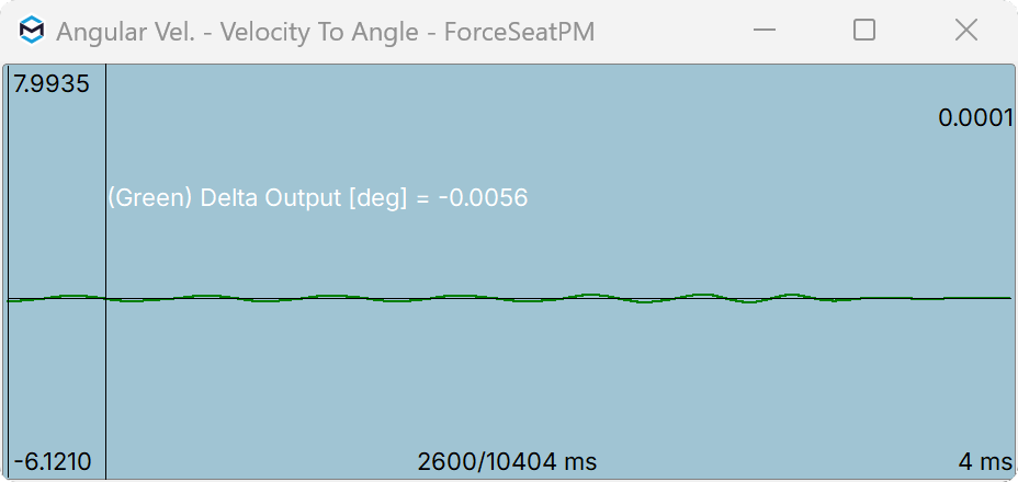
- (8) - it computes integral of angular velocity to get instantaneous angle. In other words, it uses angular velocity and time interval (4ms for 250Hz rate) between ACE loop calls to calculate angle.
θ = ∫00.004[s] ω(t) dt
Warning
The physics behind tilt coordination implies that the absolute theoretical maximum sustained lateral acceleration the motion platform is able to simulate is 1g (arcsin argument maximum value). This is for motion platform that offers 90 ° roll as work envelope. For motion platform that offers 20 ° roll, the maximum lateral acceleration is 3 [m/s□d]. For 10 ° roll, the value is limited to 1.5 [m/s□d]. If the SIM generates sustained accelerations greater than the motion platform is able to handle, Input limitation block must be used to scale down and limit the input acceleration.
3.3.1 Input limitation
This block has exactly the same function for all 3 paths, the difference is only in units.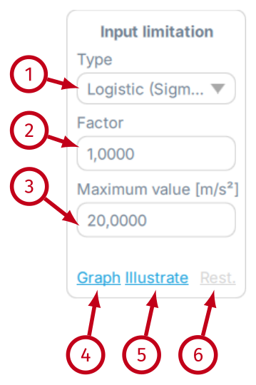
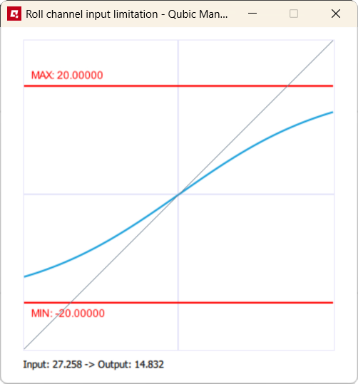
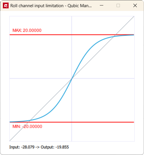
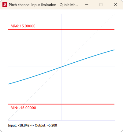
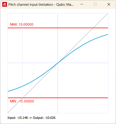
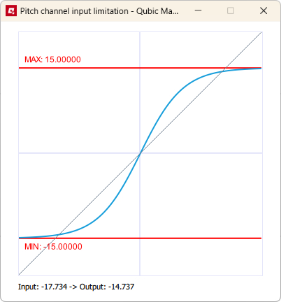
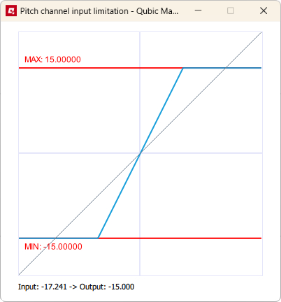
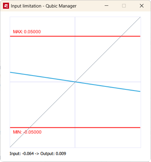
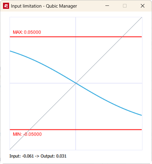
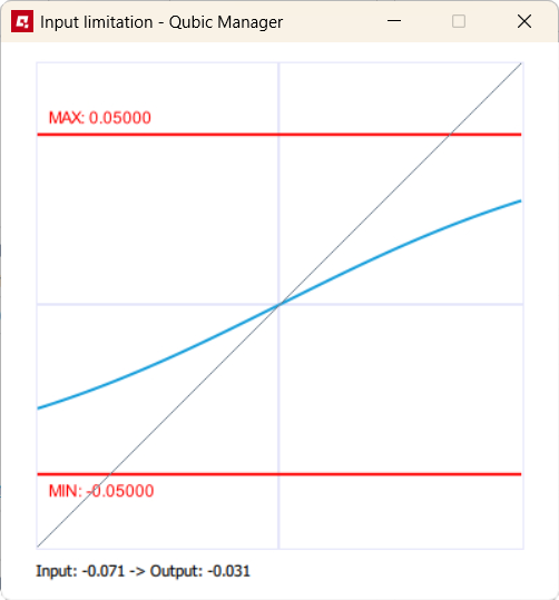
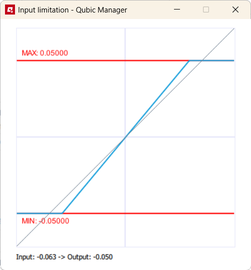
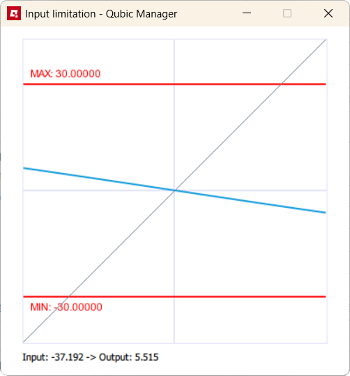
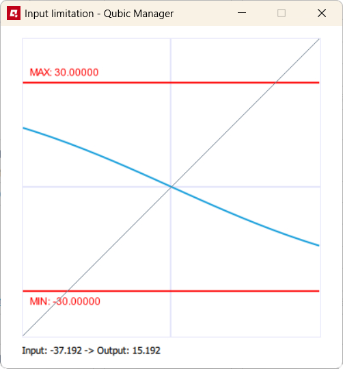
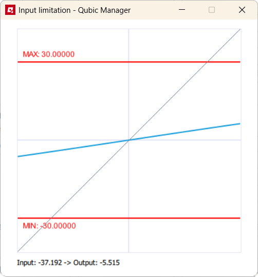
- (1) - defines type of the limitation function. Following options are available: None and Logistic. It is recommended to use Logistic as limitation function as it offers smooth close to boundaries experience. You can click Illustrate to check how Factor and Maximum value affects the input signal.
f(x) = max · (-21 + e2x · dfracfactormax + 1)
- (2) - defines first parameter for limitation function. You can click Illustrate to check how it affects the input signal. Use negative factor to inverse the signal and fix incorrect polarity.
- (3) - defines second parameter for limitation function. You can click Illustrate to check how it affects the input signal. Due to Exp function characteristic, sometimes it is necessary to use greater maximum value than normally required. You can click Illustrate to check how it affects the input signal.
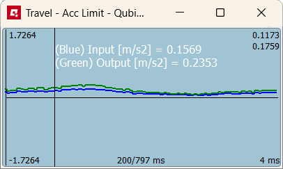
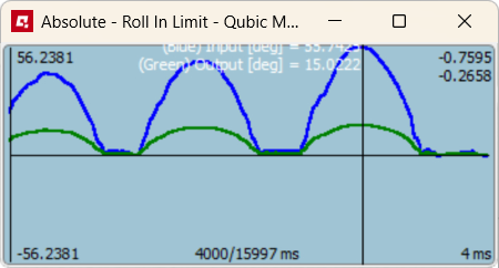
- (4) - opens a pop-up with graph that plots input (blue) and output (green) of the block. When the SIM is running in the background, you can see how Input limitation block alters the original signal.
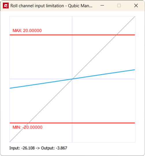
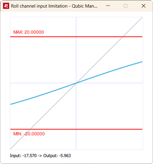
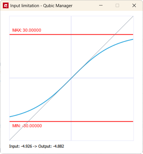
- (5) - it opens a graph that shows how the selected limitation function modifies incoming data. Use Ctrl + mouse scroll to zoom the view. Example below is for Factor = 1.5 and Maximum value = 20.
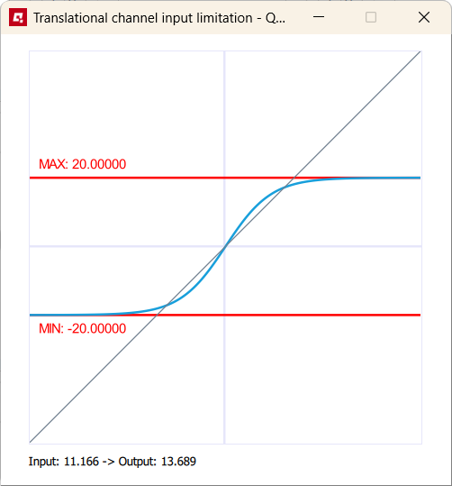
- (6) - it resets all parameters in the block to values stored in the file (recently saved).
Warning
Correct selection of Factor and Maximum value are crucial for tilt coordination component (lateral acceleration to roll transformation) to operate correctly. Input limitation together with Acceleration low-pass filter must reduce input acceleration to value which after being processed by asin and transformed into roll is within motion platform's work envelope.
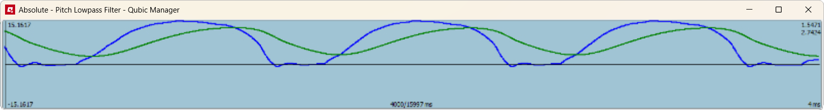
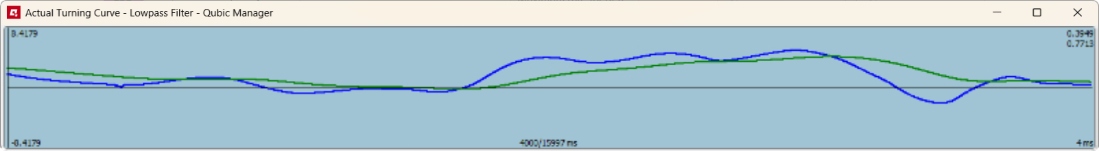
3.3.2 High-pass filter: acceleration, velocity, travel, angular velocity and angle
All high-pass filters blocks work exactly the same way. The only difference is in input data units which are irrelevant for filtering algorithm. The only required parameter is cutoff frequency [Hz].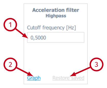
- (1) Cutoff frequency (Hz) - defines the cutoff frequency for the high-pass filter. The filter is implementation of the following formula:
yn = xn - xn - 1 - (2π f * dt - 1) * yn-12π f * dt + 1where dt is interval between calls, usually 0.004 [s], f is cutoff frequency, x is input and y is output.
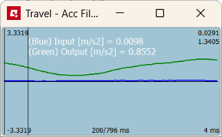
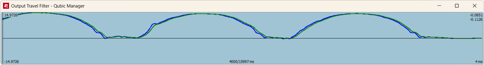
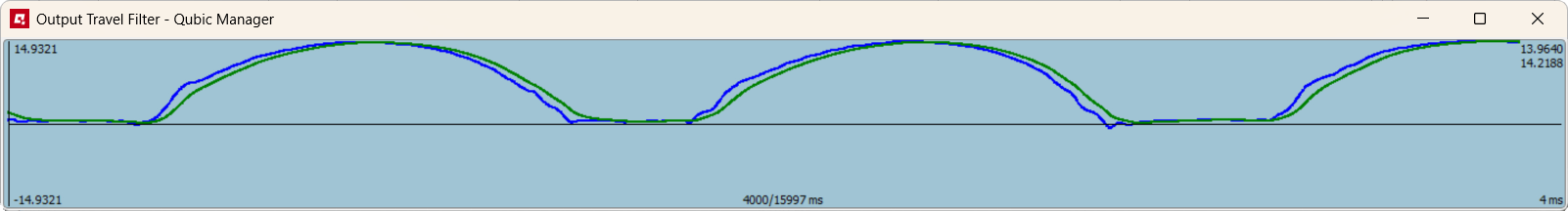
- (2) Graph - opens a pop-up with graph that plots input (blue) and output (green) of the block. When the SIM is running in the background, you can see how High-pass filter block alters the original signal.
- (3) Restore saved - resets all parameters in the block to values stored in the file (recently saved).
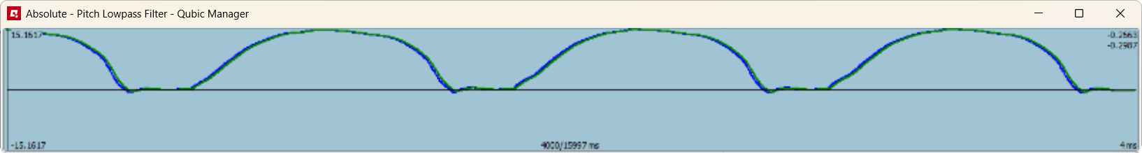
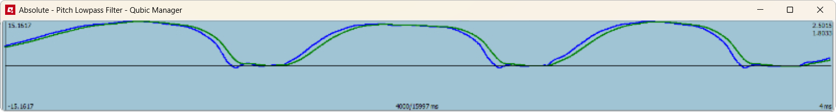
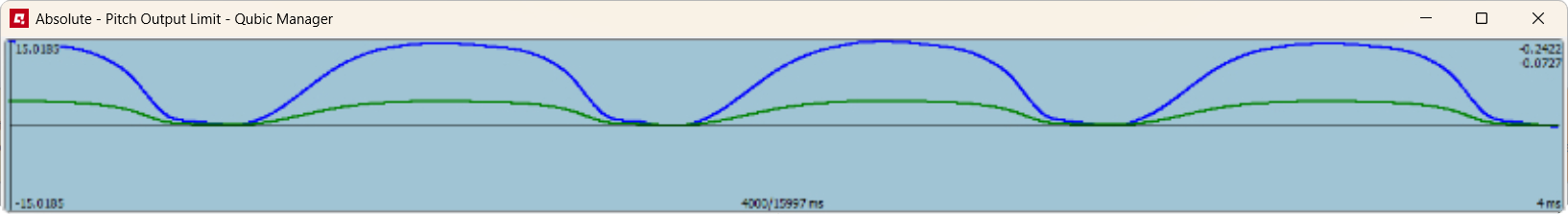
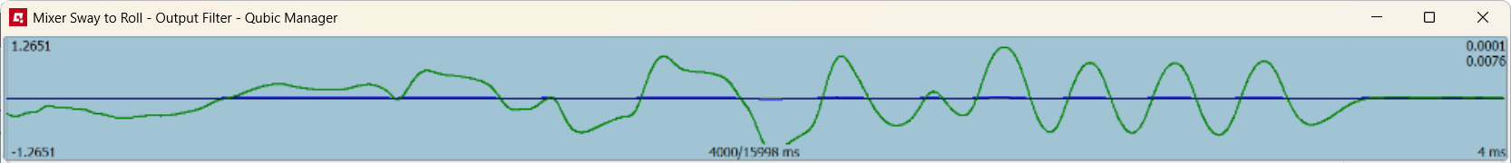
3.3.3 Output filter
Output filter block is just a filter, usually low-pass, that smooths the output data before is it being processed by the next functional block.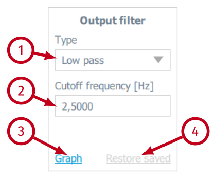
- (1) Type - defines the type of the filtering function. Following options are available: None (no output filter), Low-pass (recommended when smoothing is required).
- (2) Cutoff frequency (Hz) - defines the cutoff frequency for the Low-pass filter. It implements the following formula:
yn = x dtdt + τ + yn-1 τdt + τ, τ = 12π fwhere dt is interval between calls, usually 0.004 [s], f is cutoff frequency, x is input and y is output.
- (3) Graph - opens a pop-up with graph that plots input (blue) and output (green) of the block. When the SIM is running in the background, you can see how Output filter block alters the original signal.
- (4) Restore saved - resets all parameters in the block to values stored in the file (recently saved).
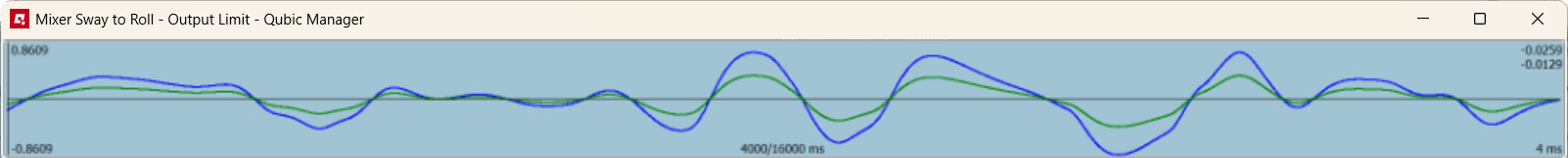
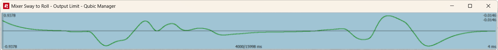
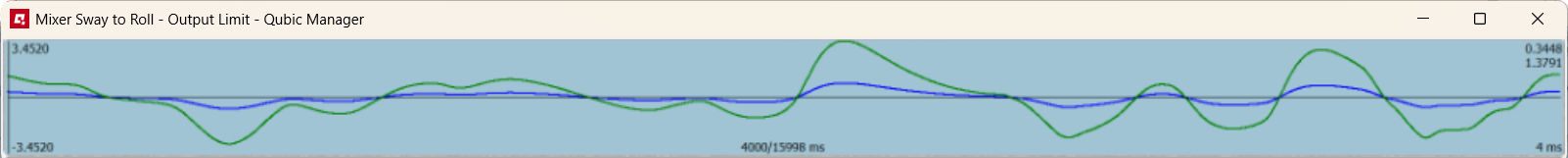
3.3.4 Limit and Angle limit
Limit and Angle limit blocks work the same way as Input limitation block with two main differences:- they are used on output data, NOT on input data;
- the maximum value is read automatically from the connected motion platform and cannot be changed.
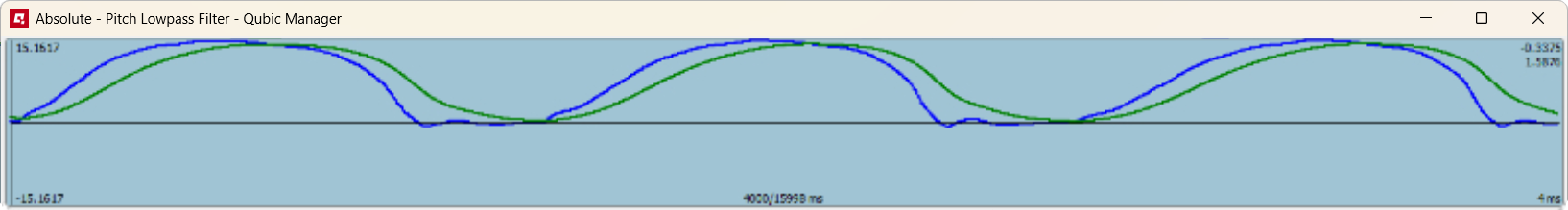
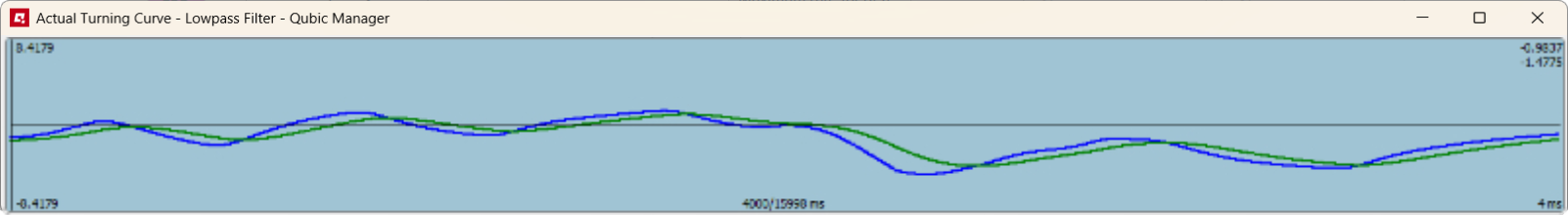
3.3.5 Acceleration low-pass filter
This low-pass filter is used only in tilt coordination path and its role is to smoothen sustained acceleration before it is transformed into rotation.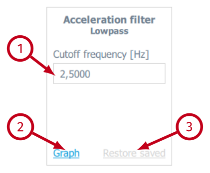
- (1) Cutoff frequency (Hz) - defines the cutoff frequency for the low-pass filter. The filter implements the following formula:
yn = x dtdt + τ + yn-1 τdt + τ, τ = 12π fwhere dt is interval between calls, usually 0.004 [s], f is cutoff frequency, x is input and y is output.
- (2) Graph - opens a pop-up with graph that plots input (blue) and output (green) of the block. When the SIM is running in the background, you can see how filter block alters the original signal.
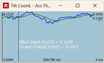
- (3) Restore saved - resets all parameters in the block to values stored in the file (recently saved).
3.3.6 Angle rate limit
Tilt coordination uses the fact that the vestibular system cannot distinguish between inertia force produced by a linear acceleration and the effect of gravity. Since humans are very sensitive to the tilt rate, the rate should be within user's perception threshold. Good starting point is 2∼4 [°/s], however very often this value is too limited to reproduce a realistic driving simulation and has to be tuned (increased). This block allows to configure tilt rate with Maximum rate parameter.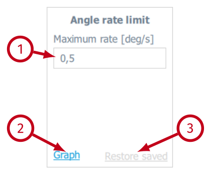
- (1) Maximum rate (deg/s) - defines maximum tilt rate. The block implements following generic (simplified for better readability) formula:
yn= yn-1 + rate · dt, if xn ≥ yn-1 + rate · dtwhere dt is interval between calls, usually 0.004 [s], rate is the maximum rate, x is input and y is output.
yn-1 - rate · dt, if xn ≤ yn-1 - rate · dt
xn, otherwise - (2) Graph - opens a pop-up with graph that plots input (blue) and output (green) of the block. When the SIM is running in the background, you can see how Angle rate limit block alters the original signal.
- (3) Restore saved - resets all parameters in the block to values stored in the file (recently saved).
Tip
For Acceleration Filter Lowpass general range of 0.1-10.0 Hz is advised. Filtering values act as follows:
- if 0.1 → less dynamics and less sharp
- if 10.0 → more dynamic and more sharp
- if 0.1 → less sharp and less travel
- if 10.0 → more sharp and more travel
3.4 Longitudinal acceleration and pitch rate
This view allows to configure parameters for each block of the classical washout algorithm related to longitudinal acceleration and pitch rate. Parameters and functions are analogical to Lateral acceleration and roll rate component and are described in previous chapter.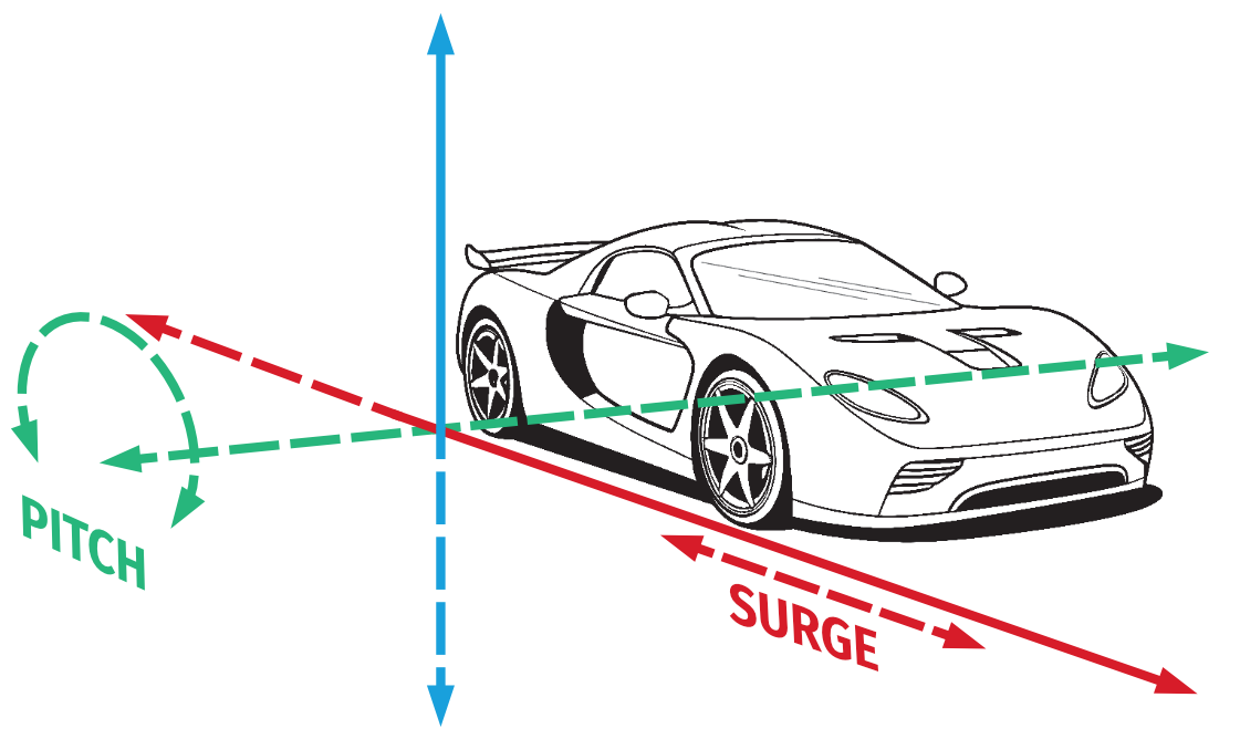
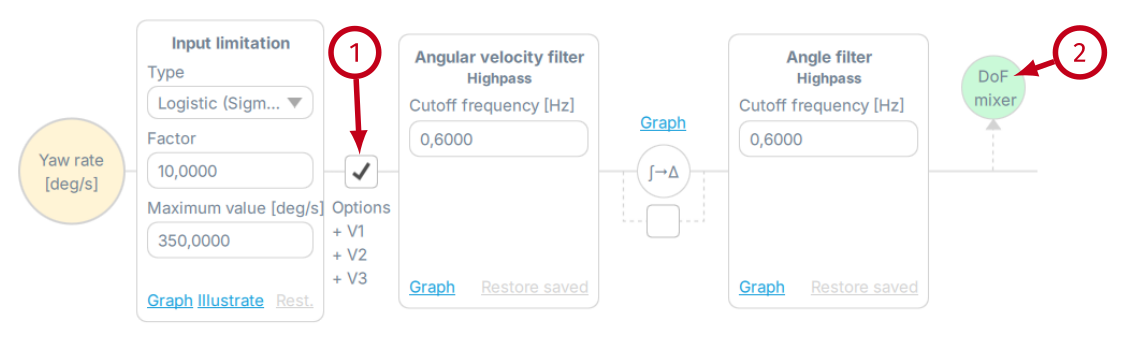
3.5 Vertical acceleration and yaw rate
Tip
For Acceleration Filter Highpass (and Angular velocity filter) general range of 0.1-10.0 Hz is advised. Filtering values act as follows:
- if 0.1 → more dynamics and more tavel
- if 10.0 → less dynamic and less travel
- if 0.1 → more dynamic and less sharp
- if 10.0 → less dynamic and more sharp
- if 0.1 → less sharp and more travel
- if 10.0 → more sharp and less travel
- if 0.1 → less sharp and less travel
- if 10.0 → more sharp and more travel
3.6 Body roll and pitch
This view allows to configure parameters for body roll and pitch. As opposed to Longitudinal and Lateral acceleration and pitch rate which imitates G-forces, body pitch and body roll translates vehicle in-game position in relation to x and z axis into platform sustained angled position (e.g. on a hill or a steep banked turn or flight sim during turn inclination).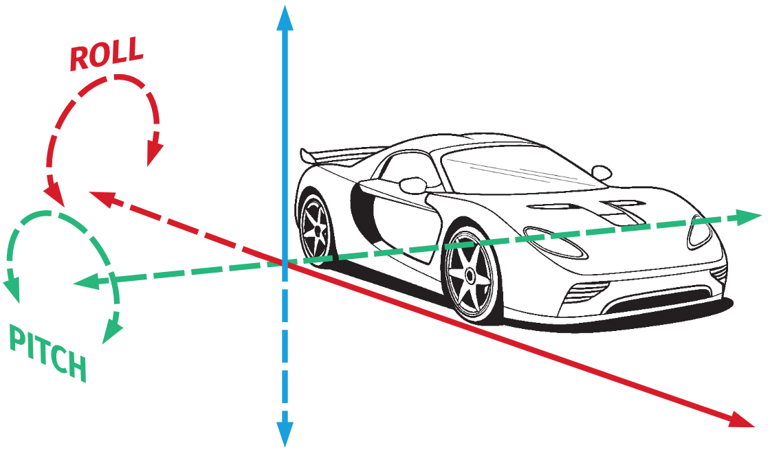
3.6.1 Body roll
This parameter allows for sustained body roll configuration (e.g. vehicle on a steep banked turn). It is combined of input signal limitation, output filter and output limit.Info
Modifying settings has an instant effect on platform's motion characteristic as long as the changes are saved (right top tab in ACE window or keyboard shortcut "CTRL+S").
3.6.2 Input limitation
Input limitation options block adjusts telemetry data from the game/simulation before it is translated into output data for the platform.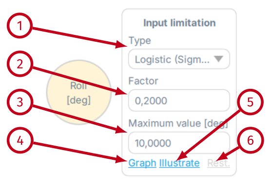
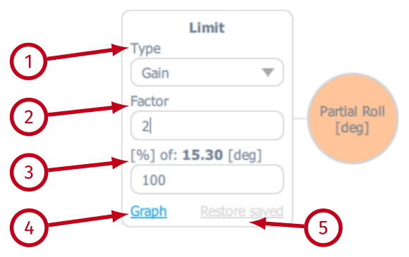
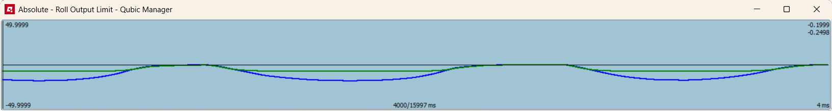
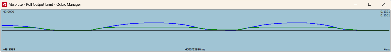
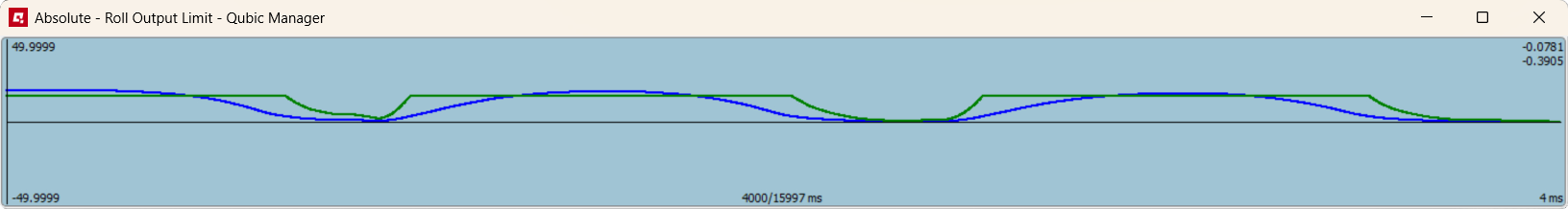
- (1) Type: none - no limitation. Type: gain - more intense input with abrupt freeze at endpoint. Type: exp - exponential increase or decrease of the input data.
- (2) Factor - overall signal gain, exponentially increases (or decreases) input data from the game/simulation (visualized in "Illustrate"). Set to negative inverts the input data.
- (3) Maximum value [deg]: limits the input data on a maximum available degree angle (visualized in "Illustrate").
- (4) Graph - opens a pop-up with graph that plots input (blue) and output (green) data of the block. When the SIM is running in the background, you can see how Input limitation block alters the original signal.
- (5) Illustrate - opens up a graph that shows how the Factor (blue line) and Maximum value (red lines) limitation function modifies incoming data. Use Ctrl + mouse scroll to zoom the view. Below are examples of Factor exponential increase. From the left: 0.15, 0.35, 0.7, 2.0 and Maximum value in degrees = 20
- (6) Rest. - restores all parameters in the block from a previously saved file.
3.6.3 Output filter
Output filter block is just a filter that smooths out or sharpens the output data before it is being processed by the next functional block.
- (1) Type - defines the type of the filtering function. Following options are available: None (no output filter), Low-pass (recommended when smoothing is required).
- (2) Cutoff frequency (Hz) - defines the cutoff frequency for the Low-pass filter. It implements the following formula:
yn = x dtdt + τ + yn-1 τdt + τ, τ = 12π fwhere dt is interval between calls, usually 0.004 [s], f is cutoff frequency, x is input and y is output.
- (3) Graph - opens a pop-up with graph that plots input (blue) and output (green) of the block. When the SIM is running in the background, you can see how Output filter block alters the original signal.
- (4) Restore saved - resets all parameters in the block to values stored in the file (recently saved).
- Low-pass cutoff frequency - 2.0 Hz
- Low-pass cutoff frequency - 1.0 Hz
- Low-pass cutoff frequency - 0.3 Hz
- Low-pass cutoff frequency - 0.1 Hz
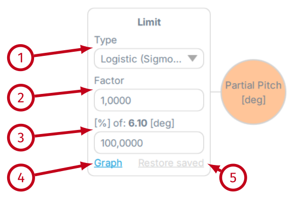
3.6.4 Limit
Limit block works the same way as Input limitation block with two main differences:- they are used on output data, NOT on input data;
- the maximum value is read automatically from the connected motion platform and cannot be changed.
- (1) Type - defines the type of the limiting function. Following options are available: None (no limitation), Gain (more intense output with abrupt freeze at endpoints) and Exponential (more smooth output).
- (2) Factor ‐ overall extent of the limitation on the output data.
- (3) % of maximum available degrees of sustained roll (software provides the maximum degree value automatically) - limits the output data on a maximum available degree angle.
- (4) Graph ‐ opens a pop-up with graph that plots input (blue) and output (green) data of the block. When the SIM is running in the background, you can see how output limitation block alters the original signal.
- (5) Restore saved ‐ resets all parameters in the block to values stored in the file (recently saved).
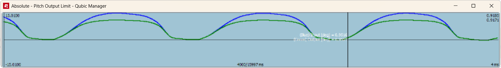
- Exponential limit, factor 0.5, 100% of degrees
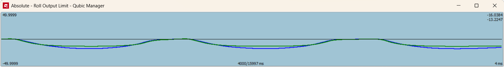
- Exponential limit, factor 0.5, 50% of degrees
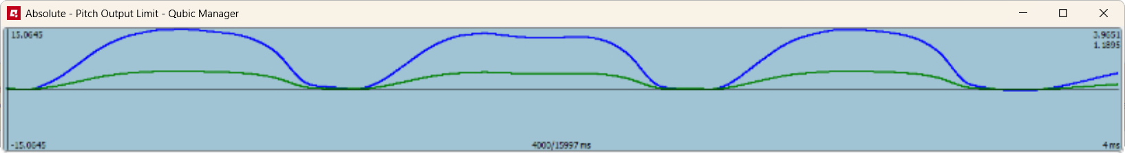
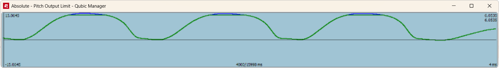
- Gain limit, factor 0.5, 100% of degrees
- Gain limit, factor 2.0, 100% of degrees
3.6.5 Body pitch
This parameter allows for sustained body pitch configuration (e.g. vehicle on a steep hill, plane diving). It is combined of input signal limitation, output filter and output limit.Info
Modifying settings has an instant effect on platform's motion characteristic as long as the changes are saved (right top tab in ACE window or keyboard shortcut "CTRL+S").
3.6.6 Input limitation
Input limitation options block adjusts telemetry data from the game/simulation before it is translated into output data for the platform.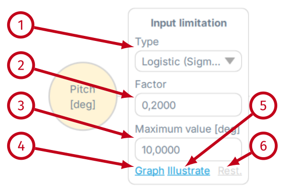
- (1) Type: none - no limitation. Type: gain - more intense input with abrupt freeze at endpoint. Type: exp - exponential increase or decrease of the input data.
- (2) Factor - overall signal gain, exponentially increases input data from the game/simulation (visualized in "Illustrate"). Set to negative inverts the input data.
- (3) Maximum value [deg]: limits the input data on a maximum available degree angle (visualized in "Illustrate").
- (4) Graph - opens a pop-up with graph that plots input (blue) and output (green) data of the block. When the SIM is running in the background, you can see how Input limitation block alters the original signal.
- (5) Illustrate - opens up a graph that shows how the Factor (blue line) and Maximum value (red lines) limitation function modifies incoming data. Use Ctrl + mouse scroll to zoom the view. Below are examples of Factor increase. From the left: exp 0.35, exp 0.8, exp 2.0, gain 2.0 and Maximum value in degrees = 15.
- (6) Rest - restores all parameters in the block from a previously saved file.
3.6.7 Output filter
Output filter block is just a filter that smooths out or sharpens the output data before it is being processed by the next functional block.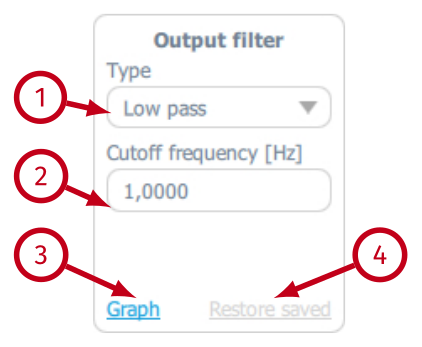
- (1) Type - defines the type of the filtering function. Following options are available: None (no output filter), Low-pass (recommended when smoothing is required).
- (2) Cutoff frequency (Hz) - defines the cutoff frequency for the Low-pass filter. It implements the following formula:
yn = x dtdt + τ + yn-1 τdt + τ, τ = 12π fwhere dt is interval between calls, usually 0.004 [s], f is cutoff frequency, x is input and y is output.
- (3) Graph - opens a pop-up with graph that plots input (blue) and output (green) of the block. When the SIM is running in the background, you can see how Output filter block alters the original signal.
- (4) Restore saved - resets all parameters in the block to values stored in the file (recently saved).
- Low-pass cutoff frequency - 4.0 Hz
- Low-pass cutoff frequency - 1.0 Hz
- Low-pass cutoff frequency - 0.35 Hz
- Low-pass cutoff frequency - 0.15 Hz
3.6.8 Limit
Limit block works the same way as Input limitation block with two main differences:- they are used on output data, NOT on input data;
- the maximum value is read automatically from the connected motion platform and cannot be changed.
- (1) Type - defines the type of the limiting function. Following options are available: None (no limitation), Gain (more intense output with abrupt freeze at endpoints) and Exponential (more smooth output).
- (2) Factor ‐ overall extent of the limitation on the output data.
- (3) % of maximum available degrees of sustained pitch (software provides the maximum degree value automatically) - limits the output data on a maximum available degree angle.
- (4) Graph ‐ opens a pop-up with graph that plots input (blue) and output (green) data of the block. When the SIM is running in the background, you can see how output limitation block alters the original signal.
- (5) Restore saved ‐ resets all parameters in the block to values stored in the file (recently saved).
- Exponential limit, factor 0.3, 100% of degrees
- Exponential limit, factor 1.0, 50% of degrees
- Gain limit, factor 0.3, 100% of degrees
- Gain limit, factor 1.0, 100% of degrees
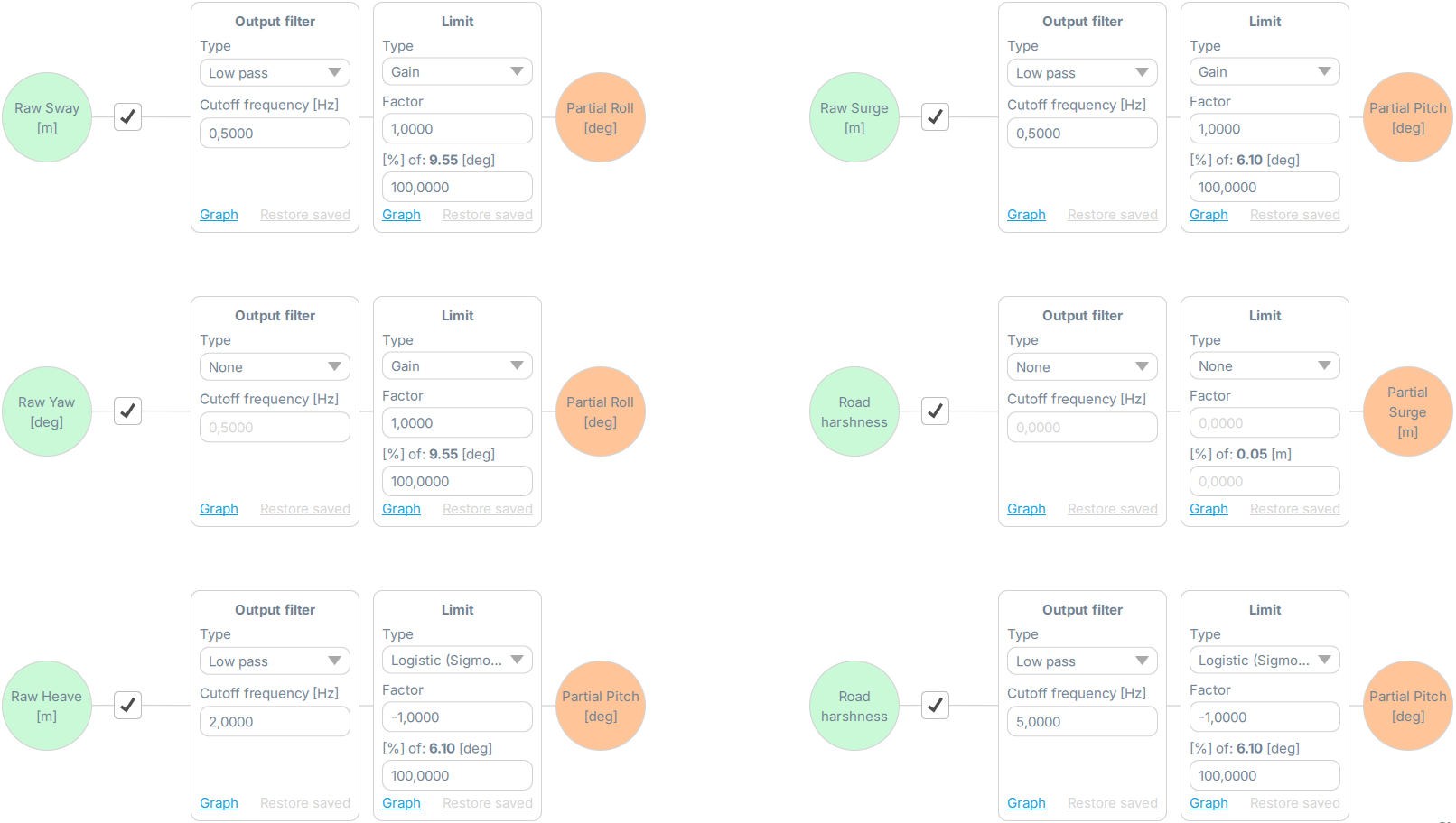
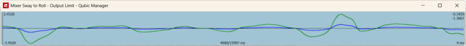
3.7 DoF mixer
This parameter allows for configuration of the substitution of a missing degree of freedom. If the motion platform lacks certain motion capability, it can be substituted with a similar one to give the impression of that movement. All of the DoF mixer parameters are independent of each other.Info
It is unnecessary to enable DoF mixer block on the platform that is already able to generate certain degree of freedom - it will be redundant with the original (raw) effect and will not affect the motion of the platform.
- Raw sway into Partial roll
- Raw yaw into Partial roll
- Raw surge into Partial pitch
- Raw heave into Partial pitch
- Road harshness into Partial pitch
- Road harshness into Partial surge
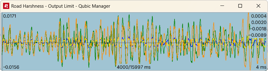
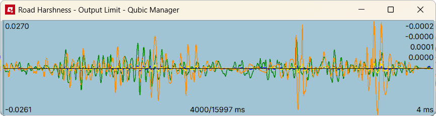
3.7.1 Output filter and limit
All parameters are combined of output filter and output limit block.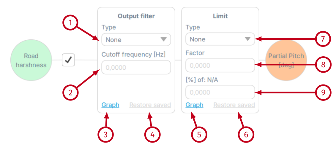
- (1) Type - defines the type of the filtering function. Following options are available: None (no limitation) and Low-pass (recommended when smoothing is required).
- (2) Cutoff frequency (Hz) - defines the cutoff frequency for the Low-pass filter. It implements the following formula:
yn = x dtdt + τ + yn-1 τdt + τ, τ = 12π fwhere dt is interval between calls, usually 0.004 [s], f is cutoff frequency, x is input and y is output.
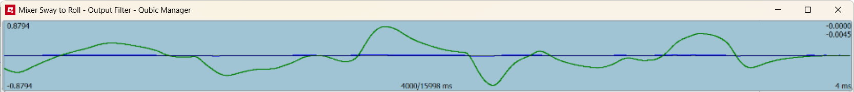
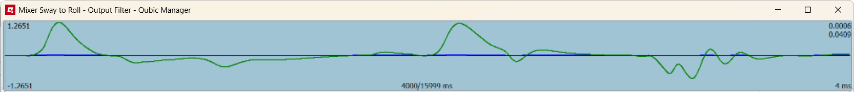
- (3) Graph ‐ opens a pop-up with graph that plots input (blue) and output (green) data of the block. When the SIM is running in the background, you can see how output limitation block alters the original signal.
- (4) Restore saved ‐ resets all parameters in the block to values stored in the file (recently saved).
- (7) Type - defines the type of the limiting function. Following options are available: None (no limitation), Gain (more intense output with abrupt freeze at endpoints) and Exponential (more smooth output).
- (8) Factor - overall extent of the limitation on the output data.
- (9) % of maximum available interval in degrees (software provides the maximum value automatically) - limits the output data on a maximum available movement.
- (5) Graph ‐ opens a pop-up with graph that plots input (blue) and output (green) data of the block. When the SIM is running in the background, you can see how output limitation block alters the original signal.
- (6) Restore saved ‐ resets all parameters in the block to values stored in the file (recently saved).
Info
Ensure that the demanded raw effect is enabled first, since it transmits input data into the DoF mixer block. For example in order for the Road harshness into partial pitch parameter to work, road harshness (from Enhancer menu) must be activated and set correctly. Open the Output filter graph to check if the input data is available (blue line).
- Low-pass cutoff frequency - 0.5 Hz
- Low-pass cutoff frequency - 1.9 Hz
- Low-pass cutoff frequency - 3.0 Hz
- Gain limit, factor 0.5, 100% of degrees
- Gain limit, factor 1.0, 100% of degrees
- Gain limit, factor 4.0, 100% of degrees
- Exponential limit, factor 4.0, 100% of degrees
3.8 Enhancer - road harshness
This parameter allows for configuration of the road harshness into intermittent heave action. In "Param set 1" it only applies to vehicles (for flight configuration e.g. landing strip harshness - go to "Param set 2" in top right corner). As opposed to Vertical acceleration it only communicates uneven texture of the road (e.g. driving over patched tarmac, over a curb, grass) and will not heave the platform to simulate change in vehicle's weight (g-force). Enhancer is an autonomous effect that can be configured with every other effect disabled.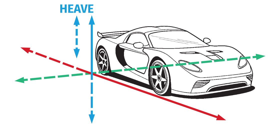
Info
Modifying settings has an instant effect on platform's motion characteristic as long as the changes are saved (right top tab in ACE window or keyboard shortcut "CTRL+S").
3.8.1 Input limitation
Input limitation options block adjusts telemetry data from the game/simulation before it is translated into output data for the platform.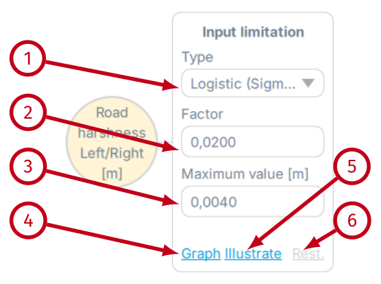
- (1) Type: none - no limitation. Type: gain - more intense input with abrupt freeze at endpoint. Type: exp - exponential increase or decrease of the input data.
- (2) Factor - overall signal gain, exponentially increases input data from the game/simulation (visualized in "Illustrate"). Set to negative inverts the input data.
- (3) Maximum value [m] - limits the input data to a specific number metres (0.XX for centimeters) number (visualized in "Illustrate").
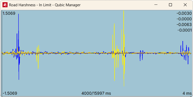
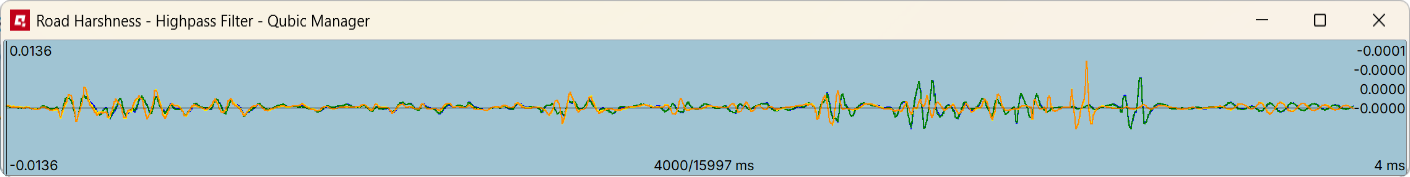
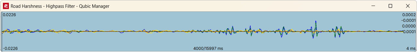
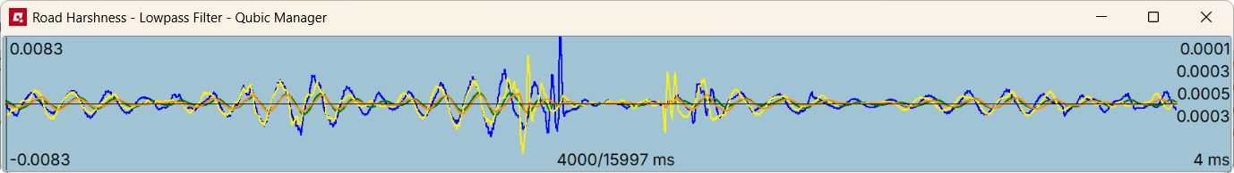
- (4) Graph - opens a pop-up with graph that plots left input (blue), right input (yellow), left output (green) and right output (orange) data of the block. When the SIM is running in the background, you can see how Input limitation block alters the original signal.
- (5) Illustrate - opens up a graph that shows how the Factor (blue line) and Maximum value (red lines) limitation function modifies incoming data. Use Ctrl + mouse scroll to zoom the view. Below are examples of Factor increase. From the left: exp -0.15, exp -0.6, exp 0.5, gain 1.2 and Maximum value in meters = 0.05 m.
- (6) Rest. - restores all parameters in the block from a previously saved file.
3.8.2 High-pass filter
High-pass filter attenuates the low-frequency components and preserves the high-frequency components. It acts as a gateway for the input data - lower cutoff frequency in high-pass means that more detailed information is preserved for the next block. Higher cutoff frequency means that only the more noticeable stronger input data comes through to the next block and the details are reduced.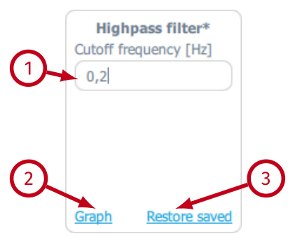
- (1) Cutoff frequency (Hz) - defines the cutoff frequency (Hz) for the high-pass filter.
- (2) Graph - opens a pop-up with graph that plots input (blue) and output (green) of the block. When the SIM is running in the background, you can see how High-pass filter block alters the original signal.
- (3) Restore saved - resets all parameters in the block to values stored in the file (recently saved).
- Cutoff frequency - 0.2 Hz
- Cutoff frequency - 0.8 Hz

- Cutoff frequency - 2.0 Hz
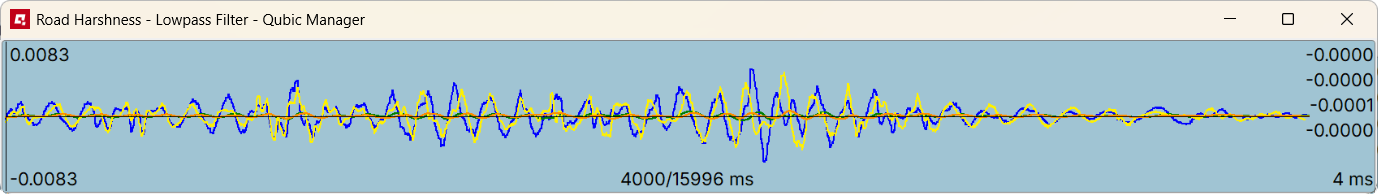
3.8.3 Output filter
Output filter block is just a filter that smooths out or sharpens the output data before it is being processed by the next functional block.
- (1) Type - defines the type of the filtering function. Following options are available: None (no output filter), Low-pass (recommended when smoothing is required).
- (2) Cutoff frequency (Hz) - defines the cutoff frequency for the Low-pass filter. It implements the following formula:
yn = x dtdt + τ + yn-1 τdt + τ, τ = 12π fwhere dt is interval between calls, usually 0.004 [s], f is cutoff frequency, x is input and y is output.
- (3) Graph - opens a pop-up with graph that plots input (blue) and output (green) of the block. When the SIM is running in the background, you can see how Output filter block alters the original signal.
- (4) Restore saved - resets all parameters in the block to values stored in the file (recently saved).
- Low-pass cutoff frequency - 4.0 Hz
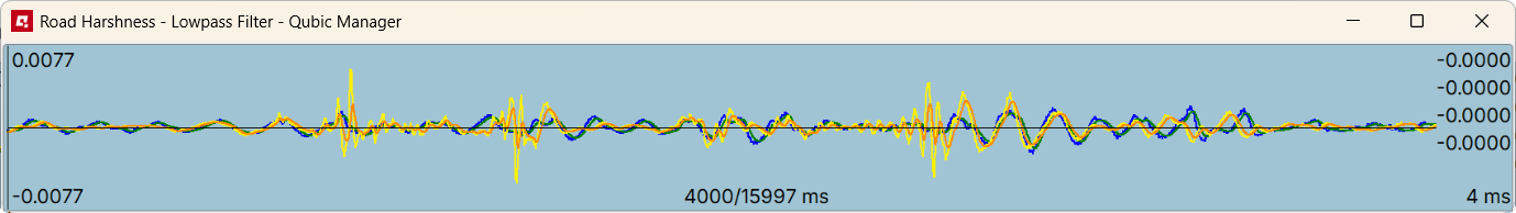
- Low-pass cutoff frequency - 1.0 Hz
- Low-pass cutoff frequency - 0.3 Hz
3.8.4 Limit
Limit block works the same way as Input limitation block with two main differences:- they are used on output data, NOT on input data;
- the maximum value is read automatically from the connected motion platform and cannot be changed.
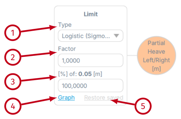
- (1) Type - defines the type of the limiting function. Following options are available: None (no limitation), Gain (more intense output with abrupt freeze at endpoints) and Exponential (more smooth output).
- (2) Factor ‐ overall extent of the limitation on the output data.
- (3) % of maximum available interval in meters (software provides the maximum degree value automatically) - limits the output data on a maximum available heave movement.
- (4) Graph ‐ opens a pop-up with graph that plots input (blue) and output (green) data of the block. When the SIM is running in the background, you can see how output limitation block alters the original signal.
- (5) Restore saved ‐ resets all parameters in the block to values stored in the file (recently saved).
- Exponential limit, factor 0.3, 100%
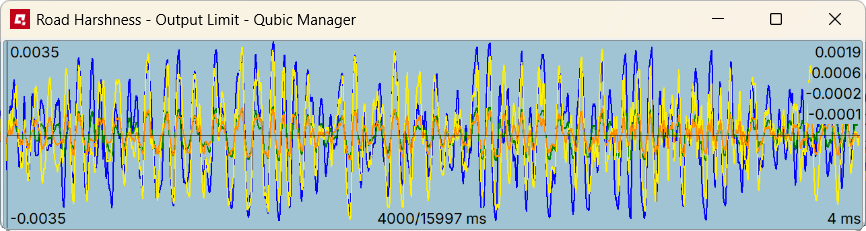
- Exponential limit, factor 1.0, 100%
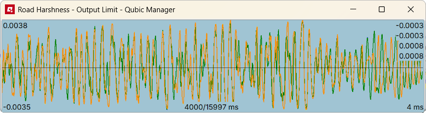
- Exponential limit, factor 5.0, 100%
- Gain limit, factor 10.0, 100%
Tip
For Highpass filter general range of 0.1-20.0 Hz is advised. Filtering values act as follows:
- if 0.1 → more travel and less dynamic
- if 20.0 → less travel and more dynamic
- if 0.1 → less sharp and less travel
- if 10.0 → more sharp and more travel
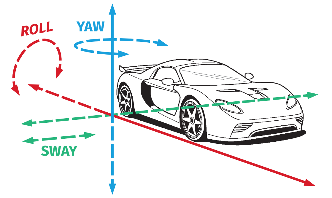
3.9 Enhancer - Side slip into Partial Yaw and Sway
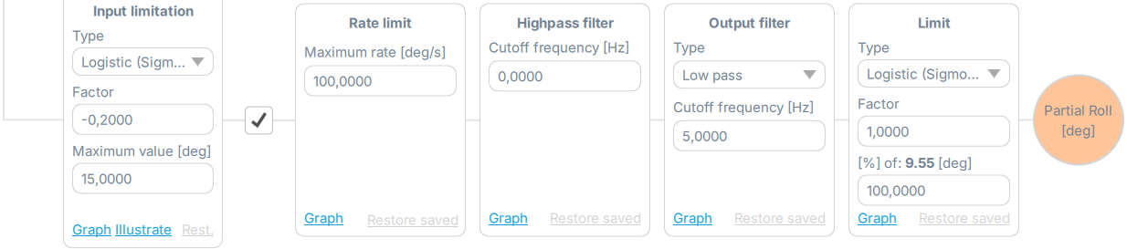
This parameter allows for configuration of side slip (oversteer grip loss) of the vehicle translated into both yaw and sway movement. It is combined of input signal limitation, rate limit, output filter and output limit. Enhancer is an autonomous effect that can be configured with every other effect disabled.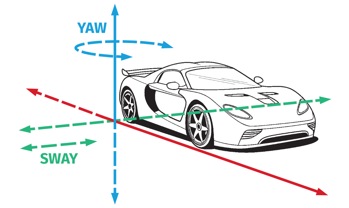
Info
Modifying settings has an instant effect on platform's motion characteristic as long as the changes are saved (right top tab in ACE window or keyboard shortcut "CTRL+S").
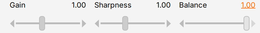
Info
Before starting configuration on sideslip parameters - Roll to yaw Balance slider must be set in QubicManager:
- For yaw configuration - set the Balance to -1
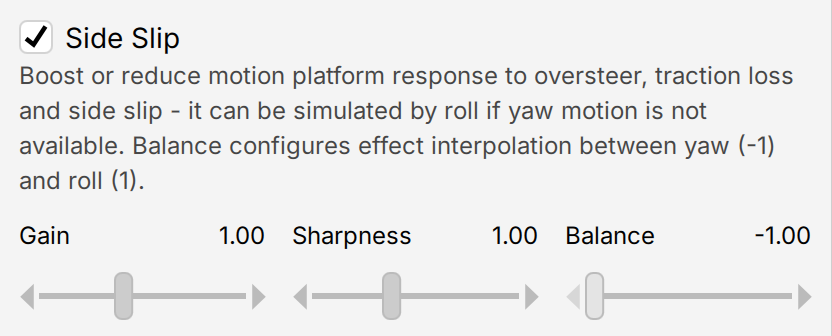
- For roll configuration - set the Balance to +1
3.9.1 Input limitation
Input limitation options block adjusts telemetry data from the game/simulation before it is translated into output data for the platform.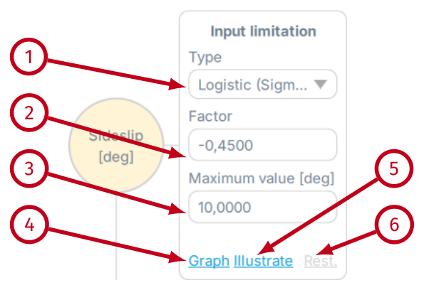
- (1) Type: none - no limitation. Type: gain - more intense input with abrupt freeze at endpoint. Type: exp - exponential increase or decrease of the input data.
- (2) Factor - overall signal gain, exponentially increases input data from the game/simulation (visualized in "Illustrate"). Set to negative inverts the input data.
- (3) Maximum value [deg]: limits the input data on a maximum available degree angle (visualized in "Illustrate").
- (4) Graph - opens a pop-up with graph that plots input (blue) and output (green) data of the block. When the SIM is running in the background, you can see how Input limitation block alters the original signal.
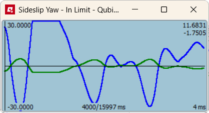
- (5) Illustrate - opens up a graph that shows how the Factor (blue line) and Maximum value (red lines) limitation function modifies incoming data. Use Ctrl + mouse scroll to zoom the view. Below are examples of Factor increase. From the left: exp -0.15, exp -0.45, exp 0.15, exp 1.0 and Maximum value in degrees = 30
- (6) Rest - restores all parameters in the block from a previously saved file.
3.9.2 Rate limit
Rate limit configures the output velocity of platform movement during a side slip event in degrees per second. The higher the value, the quicker is the platform's movement.
- (1) Maximum rate (deg/s) - overall velocity gain of platform yaw and sway movement.
- (2) Graph - opens a pop-up with graph that plots only the output (green) data of the block.
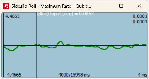
- (3) Restore saved ‐ resets all parameters in the block to values stored in the file (recently saved).
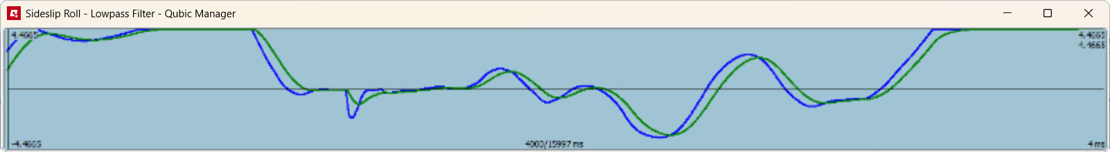
3.9.3 Output filter
Output filter block is just a filter that smooths out or sharpens the output data before it is being processed by the next functional block.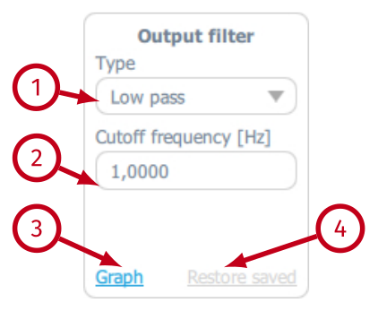
- (1) Type - defines the type of the filtering function. Following options are available: None (no output filter), Low-pass (recommended when smoothing is required).
- (2) Cutoff frequency (Hz) - defines the cutoff frequency for the Low-pass filter. It implements the following formula:
yn = x dtdt + τ + yn-1 τdt + τ, τ = 12π fwhere dt is interval between calls, usually 0.004 [s], f is cutoff frequency, x is input and y is output.
- (3) Graph - opens a pop-up with graph that plots input (blue) and output (green) of the block. When the SIM is running in the background, you can see how Output filter block alters the original signal.
- (4) Restore saved - resets all parameters in the block to values stored in the file (recently saved).
- Low-pass cutoff frequency - 0.2 Hz
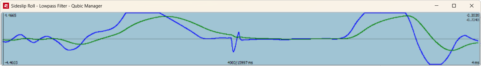
- Low-pass cutoff frequency - 0.9 Hz
- Low-pass cutoff frequency - 3.0 Hz
- Low-pass cutoff frequency - 10.0 Hz
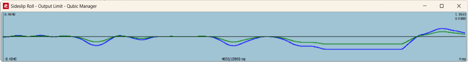
3.9.4 Limit
Limit block works the same way as Input limitation block with two main differences:- they are used on output data, NOT on input data;
- the maximum value is read automatically from the connected motion platform and cannot be changed.
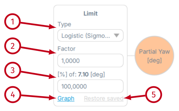
- (1) Type - defines the type of the limiting function. Following options are available: None (no limitation), Gain (more intense output with abrupt freeze at endpoints) and Exponential (more smooth output).
- (2) Factor ‐ overall extent of the limitation on the output data.
- (3) % of maximum available degrees of yaw (software provides the maximum degree value automatically) - limits the output data on a maximum available degree angle.
- (4) Graph ‐ opens a pop-up with graph that plots input (blue) and output (green) data of the block. When the SIM is running in the background, you can see how output limitation block alters the original signal.
- (5) Restore saved ‐ resets all parameters in the block to values stored in the file (recently saved).
- Exponential limit, factor 0.3, 100% of degrees
- Exponential limit, factor 1.0, 50% of degrees
- Exponential limit, factor 3.0, 100% of degrees
- Exponential limit, factor 6.0, 100% of degrees
Info
Ensure that the settings are balanced correctly and not set too high - the effect will become unpleasant for the user and the sideslip configuration can activate platform's movement even before the in-game vehicle looses traction, which will be misleading.
3.9.5 Pivot point
Pivot point configuration allows for moving the static point forward and modifying the movement geometry characteristic. This setting must be matched precisely into different motion platforms since they are constructed differently.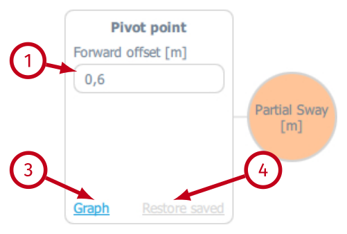
- (1) Forward offset (m) - distance of center pivot point shift forward in meters.
- (2) Graph - opens a pop-up with graph that plots input (blue) and output (green) data of the block. When the SIM is running in the background, you can see how the pivot point setting alters the original signal.
- (3) Restore saved ‐ resets all parameters in the block to values stored in the file (recently saved).

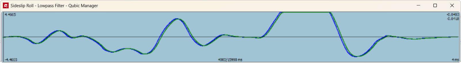
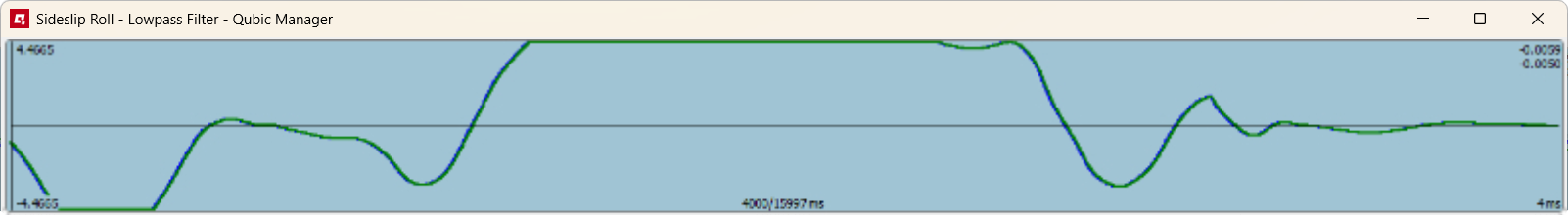
3.9.6 Sideslip into partial roll
Tip
For Angle Rate Limit a maximum value is generally a better choice - 100 deg/s.
For the Output Filter general range of 0.1-10.0 Hz is advised. Filtering values act as follows:
- if 0.1 → less sharp and less travel
- if 10.0 → more sharp and more travel
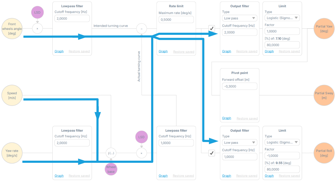
3.10 Understeer
This parameter allows for configuration of understeer grip loss (front wheels) of the vehicle translated into both yaw, sway and roll movement. It is combined of low-pass filters, rate limit, output filters and output limits.Info
Mathematical formula for Understeer is:
Understeer = frontwheelsteeringhandle - arctan(wheelbase · yawrateforwardspeed)
Info
Before starting configuration on understeer parameters - Roll to yaw Balance slider must be set in QubicManager:
- For yaw configuration - set the Balance to -1
- For roll configuration - set the Balance to +1
3.10.1 Yaw rate, speed, and front wheels angle
Low-pass filter blocks for Yaw rate, Speed, and Front wheels angle allow for filtering configuration of the input data. The Yaw rate influenced by understeer input data from game/simulation is then combined with speed and is filtered again. Front wheels angle is filtered as well and then combined with the prior mentioned.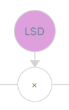
LSD stands for "Low speed dampening".
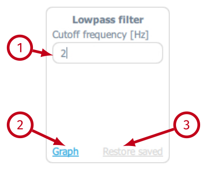
- (1) Cutoff frequency (Hz) - defines the cutoff frequency (Hz) for the low-pass filter. It implements the following formula:
yn = x dtdt + τ + yn-1 τdt + τ, τ = 12π fwhere dt is interval between calls, usually 0.004 [s], f is cutoff frequency, x is input and y is output.
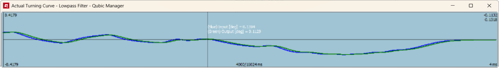
- (2) Graph - opens a pop-up with graph that plots input (blue) and output (green) of the block. When the SIM is running in the background, you can see how Low-pass filter block alters the original signal.
- (3) Restore saved - resets all parameters in the block to values stored in the file (recently saved).
- Low-pass cutoff frequency - 1.0 Hz
- Low-pass cutoff frequency - 0.3 Hz
- Low-pass cutoff frequency - 0.1 Hz
3.10.2 Rate limit
Rate limit configures the output velocity of platform movement during an understeer event in degrees per second. The higher the value, the quicker is the platform's movement.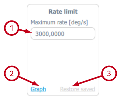
- (1) Maximum rate (deg/s) - overall velocity gain of platform yaw, sway and roll movement.
- (2) Graph - opens a pop-up with graph that plots only the output (green) data of the block.
- (3) Restore saved ‐ resets all parameters in the block to values stored in the file (recently saved).
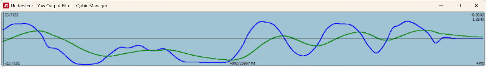
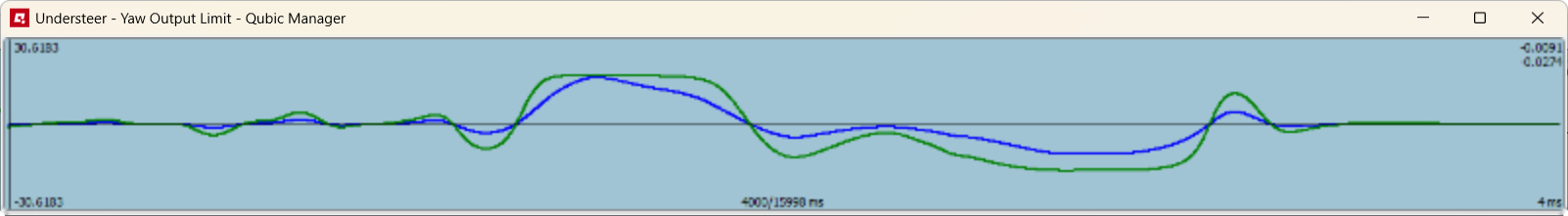
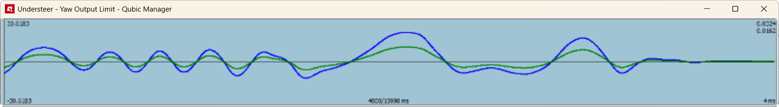
3.10.3 Understeer into yaw and sway - output low-pass filter
Output filter block is just a filter that smooths out or sharpens the output data before it is being processed by the next functional block.
- (1) Type - defines the type of the filtering function. Following options are available: None (no output filter), Low-pass (recommended when smoothing is required).
- (2) Cutoff frequency (Hz) - defines the cutoff frequency for the Low-pass filter. It implements the following formula:
yn = x dtdt + τ + yn-1 τdt + τ, τ = 12π fwhere dt is interval between calls, usually 0.004 [s], f is cutoff frequency, x is input and y is output.
- (3) Graph - opens a pop-up with graph that plots input (blue) and output (green) of the block. When the SIM is running in the background, you can see how Output filter block alters the original signal.
- (4) Restore saved - resets all parameters in the block to values stored in the file (recently saved).
- Low-pass cutoff frequency - 3.0 Hz
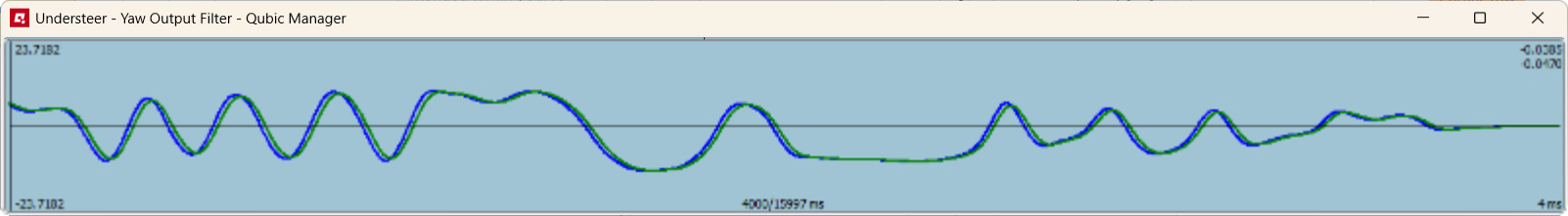
- Low-pass cutoff frequency - 0.9 Hz
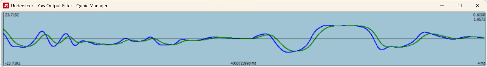
- Low-pass cutoff frequency - 0.15 Hz
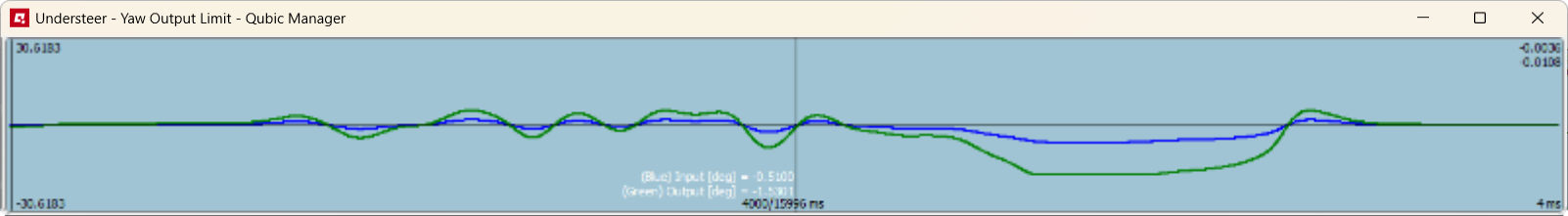
3.10.4 Understeer into yaw and sway - limit
Limit block works the same way as Input limitation block with two main differences:- they are used on output data, NOT on input data;
- the maximum value is read automatically from the connected motion platform and cannot be changed.
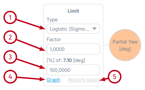
- (1) Type - defines the type of the limiting function. Following options are available: None (no limitation), Gain (more intense output with abrupt freeze at endpoints) and Exponential (more smooth output).
- (2) Factor ‐ overall extent of the limitation on the output data.
- (3) % of maximum available degrees of yaw (software provides the maximum degree value automatically) - limits the output data on a maximum available degree angle.
- (4) Graph ‐ opens a pop-up with graph that plots input (blue) and output (green) data of the block. When the SIM is running in the background, you can see how output limitation block alters the original signal.
- (5) Restore saved ‐ resets all parameters in the block to values stored in the file (recently saved).
- Exponential limit, factor 0.15, 80% of degrees
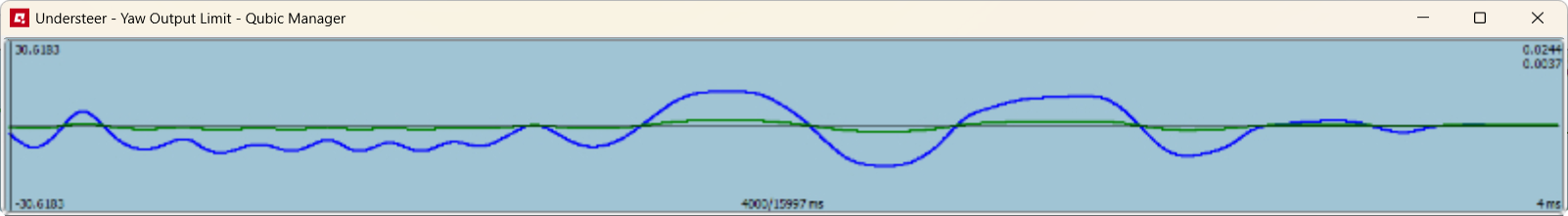
- Exponential limit, factor 3.0, 80% of degrees
- Gain limit, factor 0.5, 80% of degrees
- Gain limit, factor 3.0, 80% of degrees
Info
Ensure that the settings are balanced correctly and not set too high - the effect will become unpleasant for the user and the understeer configuration can activate platform's movement even before the in-game vehicle looses traction, which will be misleading.
3.10.5 Pivot point
Pivot point configuration allows for moving the static point forward and extending the simulation of oversteer. Also it must match every motion platform's dimensions since they are build differently.
- (1) Forward offset (m) - distance of center pivot point shift forward in meters (for backwards pivot point - set it to negative value).
- (2) Graph - opens a pop-up with graph that plots input (blue) and output (green) data of the block. When the SIM is running in the background, you can see how the pivot point setting alters the original signal.
- (3) Restore saved ‐ resets all parameters in the block to values stored in the file (recently saved).

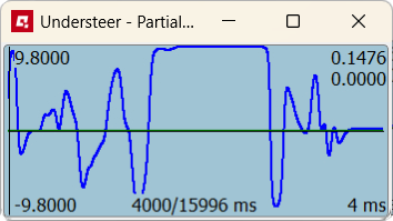
3.10.6 Understeer into roll
Partial roll action is generated the same way, as the yaw and sway action, only without the pivot point configuration. Refer to the section before the previous one for detailed information.3.11 Multiplexer
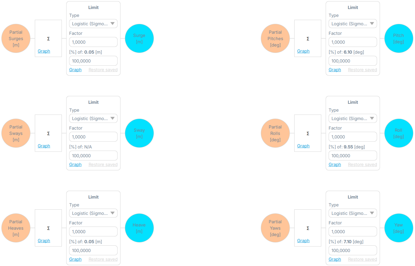
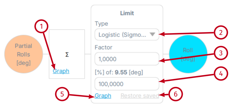
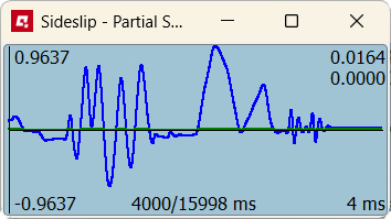
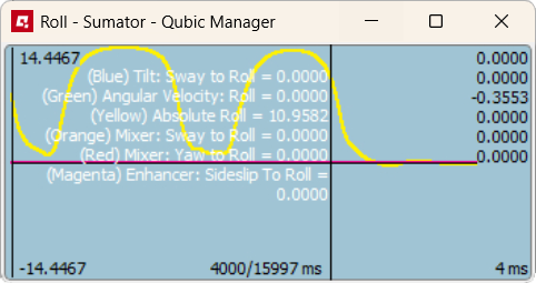
- (1) Sigma graph - opens a pop-up with graph that plots inputs from all available degrees of freedom in the platform (colors are described in the illustration below). When the SIM is running in the background, you can see how the input signal draws the line on the graph.
- (2) Type - defines the type of the limiting function. Following options are available: None (no limitation), Gain (more intense output with abrupt freeze at endpoints) and Exponential enables
- (2) Factor ‐ overall extent of the limitation on the output data.
- (3) % of maximum available angle degree (software provides the maximum degree value automatically) - limits the output data on a maximum available movement.
- (4) Graph ‐ opens a pop-up with graph that plots input (blue) and output (green) data of the block. When the SIM is running in the background, you can see how output limitation block alters the original signal.
- (5) Restore saved ‐ resets all parameters in the block to values stored in the file (recently saved).
3.11.1 Example of use - partial rolls into roll
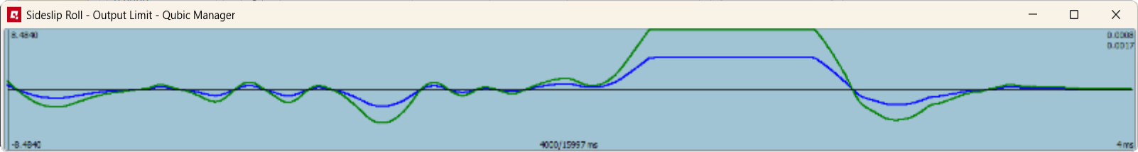
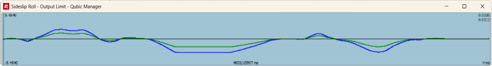
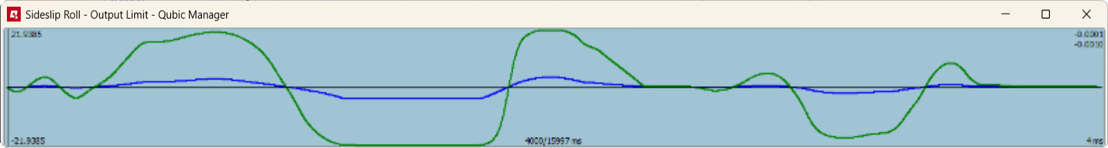
Since all of mentioned parameters are adjusted in an identical way - body roll will serve as an example. In order to better understand the output limit influence on output signal, refer to illustrations below (blue is input data, green is output data):- Exponential limit, factor 1.5, 100% of degrees
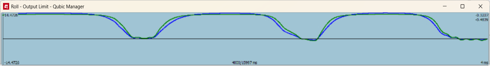
- Exponential limit, factor 1.5, 35% of degrees
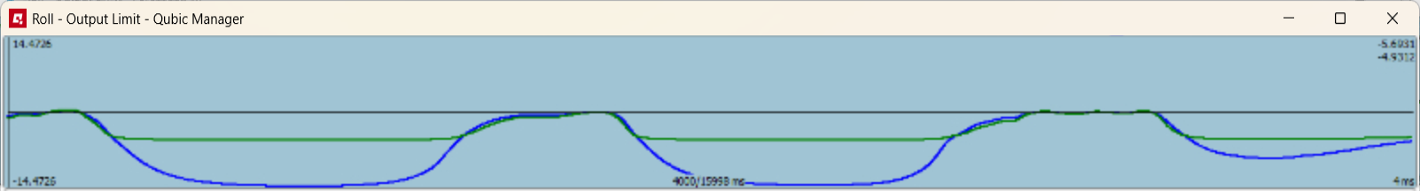
- Exponential limit, factor 0.5, 100% of degrees
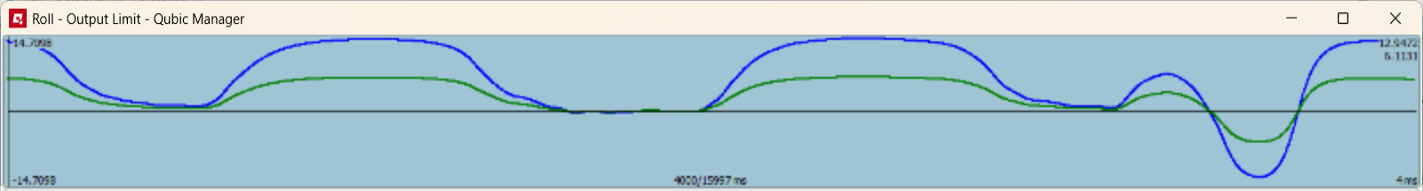
- Gain limit, factor 0.5, 100% of degrees
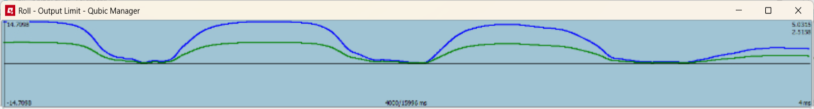
- Gain limit, factor 1.5, 100% of degrees
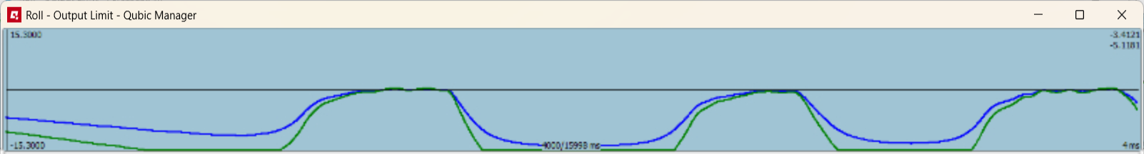
- Type: none
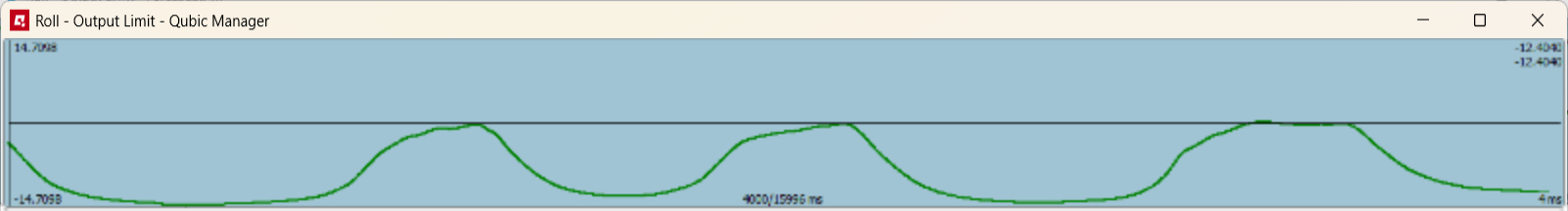
3.12 Options
All global options can be found in the Options tab.Info
All changes must be saved in order for them to take effect.
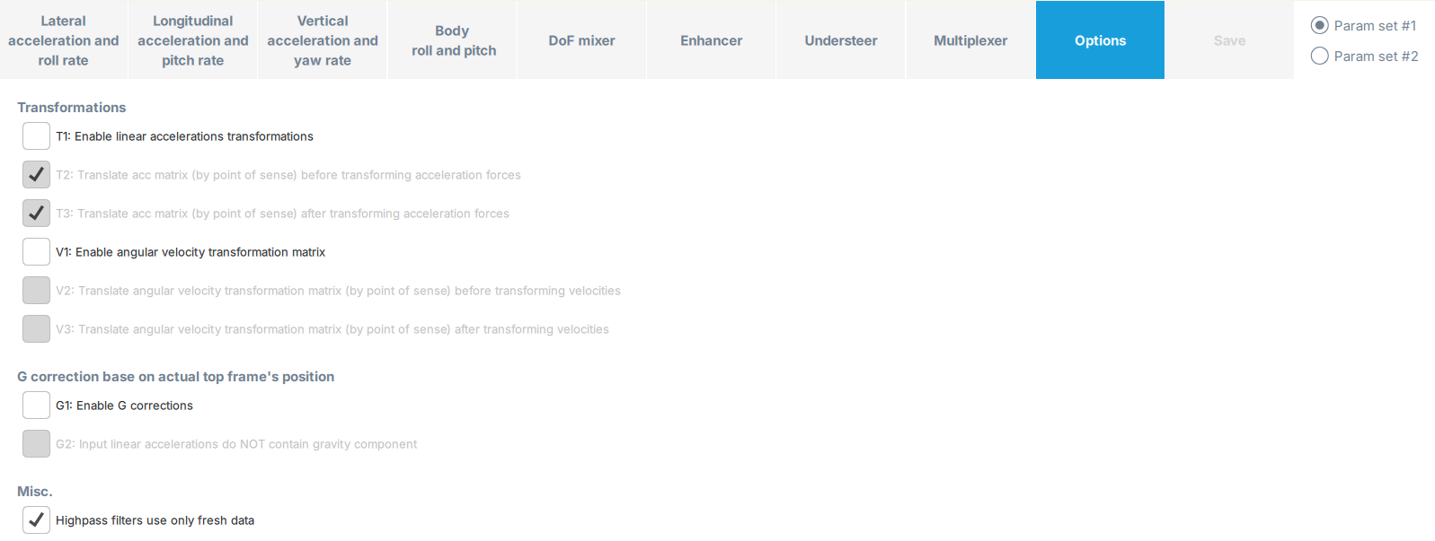
3.12.1 T1: Enable linear accelerations transformations
When this option is enabled, the input linear accelerations vector is transformed by the current top frame orientation - roll, pitch and yaw output from previous ACE run.
a2 = R1 · a1
R1 is rotation matrix generated from the most recent top table roll, pitch and yaw. a1 is a vector containing input linear accelerations. a2 is a vector containing transformed linear accelerations that is going to be used for further processing.
ax = [alongitudinal
alateral
avertical], R1 =[r1r2r30
r4r5r60
r7r8r90
0001
]
alateral
avertical], R1 =[r1r2r30
r4r5r60
r7r8r90
0001
]
3.12.2 T2/T3: Translate acceleration matrix by point of sense
Both T2 and T3 have to be turned on to enable point of sense shift for liner accelerations.3.12.3 V1: Enable angular velocity transformation
When this option is enabled, the input angular velocities vector is transformed by the current top frame orientation - roll and pitch (yaw is not used here) output from previous ACE run.
ω2 = R2 · ω1
R2 is rotation matrix generated from the most recent top table roll and pitch. ω1 is a vector containing input angular velocities. ω2 is a vector containing transformed linear accelerations that is going to be used for further processing.
ax = [alongitudinal
alateral
avertical], R2 =[1sin(roll) tan(pitch)cos(roll) tan(pitch)0
0cos(roll)-sin(roll)0
0sin(roll)cos(pitch)cos(roll)cos(pitch)0
0001
]
alateral
avertical], R2 =[1sin(roll) tan(pitch)cos(roll) tan(pitch)0
0cos(roll)-sin(roll)0
0sin(roll)cos(pitch)cos(roll)cos(pitch)0
0001
]
3.12.4 V2/V3: Translate angular velocity transformation matrix by point of sense
Both V2 and V3 have to be turned on to enable point of sense shift for angular velocities.3.12.5 G1: Enable G correction
When this option is enabled, the gravity vector is subtracted from the linear accelerations vector (calculated by T1). The gravity vector is being calculated using current top frame orientation - roll and pitch output from previous ACE run.
a3 = a2 - g1
g1 is gravity vector generated from the most recent top table roll and pitch. a2 is a vector containing linear accelerations, transformed by T1 if it was enabled. a3 is a vector containing transformed linear accelerations that is going to be used for further processing.
ax = [alongitudinal
alateral
avertical], g1 =[9.81ms2 sin(pitch)
9.81ms2 sin(roll) cos(pitch)
9.81ms2 cos(roll) cos(pitch)
]
alateral
avertical], g1 =[9.81ms2 sin(pitch)
9.81ms2 sin(roll) cos(pitch)
9.81ms2 cos(roll) cos(pitch)
]
Tip
Using G correction is OPTIONAL and decision if this option should be enabled depends on end user preferences.
3.12.6 G2: Input linear accelerations does NOT contain gravity component
If G1 is enabled and top table roll and pitch are close to 0 (zero), the g1 vector equals to:
g1 =[0
0
9.81ms2
]
It is perfectly fine if input linear accelerations contains gravity component. Otherwise top frame and motion cues are shifted in space. G2 option helps to compensate it but removing this 1[g] constant from the gravity correction vector g1.
0
9.81ms2
]
a3 = a2 - g1 + g2
Where:
ax = [alongitudinal
alateral
avertical], g1 = [9.81ms2 sin(pitch)
9.81ms2 sin(roll) cos(pitch)
9.81ms2 cos(roll) cos(pitch)
], g2 = [0
0
9.81ms2
]
alateral
avertical], g1 = [9.81ms2 sin(pitch)
9.81ms2 sin(roll) cos(pitch)
9.81ms2 cos(roll) cos(pitch)
], g2 = [0
0
9.81ms2
]
3.12.7 Highpass filters use only fresh data
When this option is enabled, highpass filter will use input data directly from the game/simulation, instead of ForceSeat (which is transmitted at several times higher frequency). That will result in a smoother platform operation (for flight simulations mainly).4 Appendixes
4.1 Visual Studio Code as motion script editor
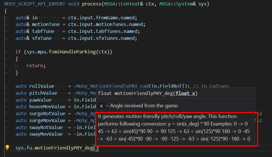
This short tutorial shows how to use Visual Studio Code to edit motion scripts associated with profiles in the ForceSeatPM. Using Visual Studio Code enables code completion (IntelliSense), syntax highlighting and contextual help. It allows also to browse API classes and functions directly from the editor.Info
This tool is NOT REQUIRED to use ACE Editor. It is useful only in cases when motion script needs to be enhanced or heavily modified.
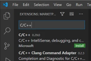
4.1.1 Installation and configuration
Download and install Visual Studio Code: https://code.visualstudio.com/. Next start the program, go to File, Preferences, Extensions and install C/C++ extension.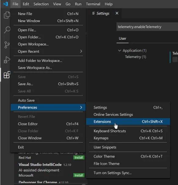
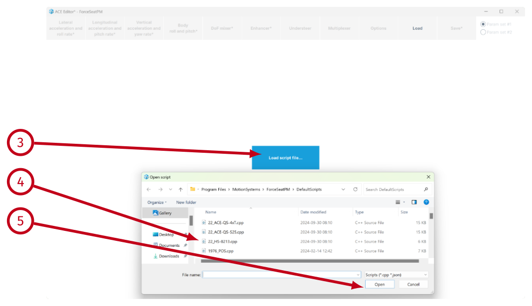
4.1.2 Usage
Clone the selected profile, e.g. SDK – Vehicle Telemetry:- disable Shallow copy
- enable Activate new profile
- enable Open editor for new profile
- enable Clone scripts
- Select Acceleration profile (1): Auto, Rapid, Balanced, Smoothest. It regulates how fast will the motion platform perform.
- Set Maximum speed of the motion platform (2) to any value - machine will not exceed that speed at any point.
- Press Run button (3) next to the script to verify that the script works correctly and there are no errors in the the output console.
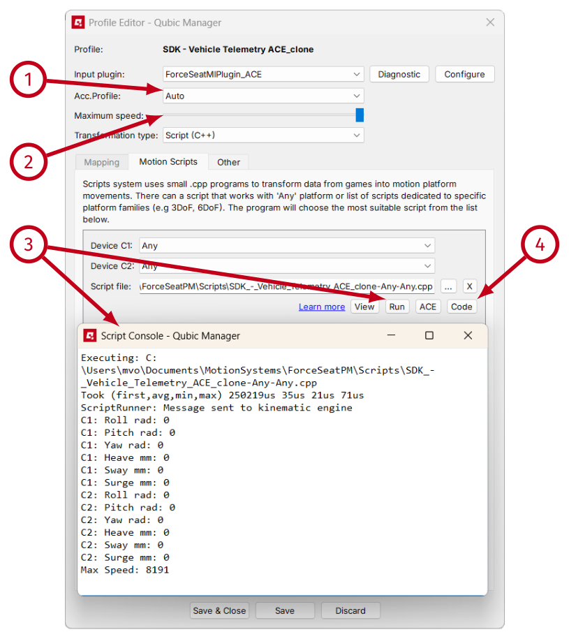
- Click Code (4) to open the script in Visual Studio Code/
- If you are editing the script when the game is running in the background and you plan to switch (Alt+Tab) to the game to check your changes (e.g. changed filter parameters) - you can close the Profile Editor. ForceSeatPM will detect any changes made to the script and reload it. If there is any syntax error in the script, details will be displayed in Action Center.
- If you are editing the script without the game running in the background or you want to check the script manually and see results in the output console, then don't close the Profile Editor - you will be clicking Run button later.
C:\Program Files (x86)\MotionSystems\ForceSeatPM\ScriptsAPI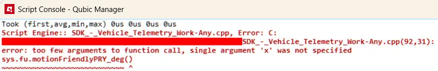
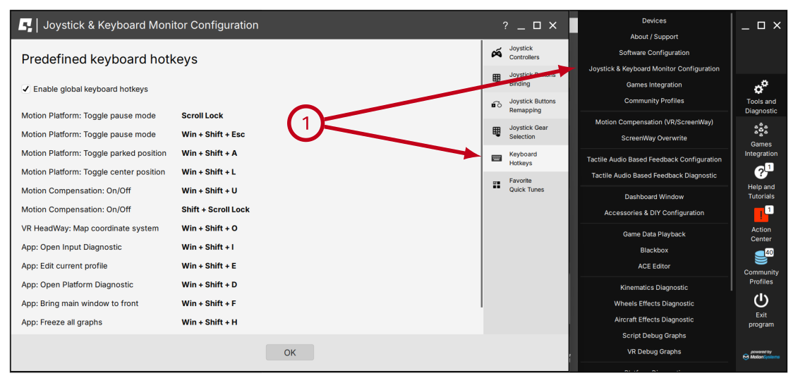
4.2 List of keyboard hotkeys
Current list of keyboard hotkeys is always displayed in the ForceSeatPM in Software Configuration. Go to Tools and Diagnostic, Software Configuration and then Keyboard Hotkeys tab. It is not possible to change keys binding, it is possible only to disable all hotkeys if they interfere with other applications.